16. Evaluation Analysis

Designing your evaluations is one of the most important aspects of any user experience process. If these evaluations are designed badly you will not be able to apply the correct analysis, and if you cannot apply the correct analysis you will not be able to make any conclusions as to the applicability or success of your interventions at the interface or interactive level [Baggini and Fosl, 2010]. In reality, this means that if this is not done correctly the previous ≈200 pages of this book have been, to a large extent, pointless.

As we shall see, good design is based upon an understanding of how data should be collected, how that data should be analysed, and how the ethical aspects of both the collection and analysis should proceed. However, the two most important aspects of any evaluation are an understanding of science, and more specifically the scientific method; and an understanding of the importance of how you select your participants (called ‘subjects’ in the old–days and still referred to as such in some current texts).

You probably think you already know what science is, how it is conducted, and how science progresses; but you are probably wrong. We will not be going very deep into the philosophy of science, but cover it as an overview as to how you should think about your evaluations and how the scientific method will help you in understanding how to collect and analyse your data; to enable you to progress your understanding of how your interventions assist users; key to this is the selection of a representative sample of participants.

Science works by the concept of generalisation – as do statistics, in which we expect to test our hypothesis by observing, recording and measuring user behaviour in certain conditions. The results of this analysis enabling us to disprove our hypothesis, or support it, thereby applying our results – collected from a small subset of the population (called a sample) – to the entirety of that population. You might find a video demonstrating this concept more helpful [Veritasium, 2013].

The way this works can be via two methods:

1. Inductive reasoning, which evaluates and then applies to the general ‘population’ abstractions of observations of individual instances of members of the same population, for example; and,
2. Deductive reasoning, which evaluates a set of premises which then necessitate a conclusion⁷ – for example: {(1) Herbivores only eat plant matter; (2) All vegetables contain only plant matter; (3) All cows are herbivores} → Therefore, vegetables are a suitable food source for Cows⁸.

Now, let’s have a look at the scientific method in a little more detail.

16.1 Scientific Bedrock

Testing and evaluation are the key enablers behind all user experience interaction work, both from a scientific and practical perspective. These twin concepts are based within a key aspect of HCI, the scientific method, and its application as a means of discovering information contained within the twin domains of human behaviour and use of the computer. It is then appropriate that you understand this key point before I move on to talking in more detail about the actual implementation of the scientific method in the form of validating your interface design.

As you may have noticed, UX takes many of its core principles from disjoint disciplines such as sociology and psychology as well as interface design and ergonomics, however, laying at its heart is empiricism⁹. The scientific landscape, certainly within the domain of the human sciences, is contingent on the concept of logical positivism. Positivism attempts to develop a principled way of approaching enquiry through a combination of empiricism, methods employed within the natural sciences, and rationalism¹⁰. The combination of empiricism (observation) and rationalism (deduction) make a powerful union that combines the best points of both to form the scientific method.

The scientific method is a body of techniques for investigation and knowledge acquisition [Rosenberg, 2012]. To be scientific, a method of inquiry must be based on the gathering of observable, empirical and measurable evidence, and be subject to specific principles of reasoning. It consists of the collection of data through observation and experimentation, and one of the first to outline the specifics of the scientific method was John Stuart Mill. Mill’s method of agreement argues that if two or more instances of a phenomenon under investigation have only one of several possible causal circumstances in common, then the circumstance in which all the instances agree is the cause of the phenomenon of interest. However, a more strict method called the indirect method of difference can also be applied. Firstly, the method of agreement is applied to a specific case of interest, and then the same principle of the agreement is applied to the inverse case of interest.

Philosophical debate has found aspects of the method to be weak and has generated additional layers of reasoning which augment the method. For instance, the concept of ‘refutability’ was first proposed by the philosopher Karl Popper. This concept suggests that any assertion made must have the possibility of being falsified (or refuted). This does not mean that the assertion is false, but just that it is possible to refute the statement. This refutability is an important concept in science. Indeed, the term ‘testability’ is related and means that an assertion can be falsified through experimentation alone.

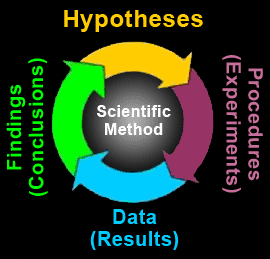
So we can see that put simply (see Figure: The Scientific Method), the scientific method enables us to test if the things we believe to be true, are in fact true. At it’s most basic the method progresses along the following lines:

1. Firstly, we create a hypothesis that, in the best case, cannot be otherwise interpreted and is ‘refutable’; for example we might make the statement ‘all swans are white’. In this case, we may have travelled widely and tried to observe swans in every country and continent in an attempt to support our hypothesis.
2. While, we may be able to amass many observations of white swans we must also realise that a statement must be refutable. If the hypothesis remains intact it must be correct; in our example, we may try to observe every swan that exists in, say, the UK, or Europe, or the Americas, which is not white.
3. However, one instance of an observation of a non-white swan will disapprove our hypothesis; in this case, when we arrive in Australia we discover a black swan, in this case, we can see all swans are not white and our hypothesis is found to be incorrect.

There have been many debates regarding the question of whether inductive reasoning leads to truth. In general, we can make some inductive leaps if they are based on good science, and these leaps may not be accurate, but may well assist us in our understanding. In the UX domain, we use mathematical (statistical) methods to help us understand these points. For example, if we collect a set of data which compares the time it takes to select a point of the screen with the mouse then we can make sure that data is valid within just the set of people who participated; this is called internal validity. However, we then want to generalise these results to enable us to say something about the wider population, here we can use well formed and tested statistical tests that enable us to mathematically generalise to a population; this is called external validity. In the human sciences, there is often no 100% certainty, all we have is a level of confidence in how a particular test relates to the population, and, therefore, how useful the knowledge generated from it is.

16.1.1 Variables

Many variable types have arisen in the human sciences methodology to enable better discussion and more accurate planning of these more controlled experiments. In general, evaluations can be characterised by the presence of a subject variable, a behavioural variable (the behavioural variables are really the user demographics, and these are really only used as part of the analysis or in participant selection to create a representative sample of the population.), a stimulus variable, and an observable response. For, the UX specialist this means that the behavioural variable can be equated to the user, the stimulus variables can be equated to the interface or the computer system, and the observable response is a thing that we often measure to understand if there is a benefit after we have manipulated the stimulus. In more detail, the subject variable discusses aspects such as the participant and the characteristics of that participant that can be used to classify them; so this would mean factors such as age, weight, gender, etc. The experimental evaluation also relies on independent and dependent variables. The confusing aspect of all of this is the same variable is sometimes named differently in different subjects; so:

• Behavioural = demographics, or subject variables, or conditions;
• stimulus = independent variable, or input, or cause; and
• response = dependent variable, or output, or effect;

The independent variable is the thing that we manipulate, in UX, this is normally an aspect of the interface that is under investigation; for instance the level of a menu item, or the position of a click button. The dependent variable is the thing that we measure, the response, in UX, this is often the response of a user interacting with the interface or system. Further, a constant is any variable that is prevented from varying and an extraneous variable is any variable other than the independent variable that might affect the dependent measure and might confound the result. Therefore, we can see that the definition of the variables along with an understanding of their presence and the means by which to control them are key to creating a well-found experimental study.

There are many different factors that may affect the internal or external validity of an experiment; called confounding variables. The effects of confounding variables can be decreased by adequate preparation of the laboratory setting for the experimental work such that participants feel comfortable; single or double blind procedures in which the UX specialist is applying the evaluation does not know the desired outcome. Or, in the case of triple blind procedures, where the practitioner applying the evaluation and the practitioner analysing the results does not know the desired outcome. Multiple observers may also be used in trying to reduce the confounding variables as well as specifically objective measures and in some cases automation of the process. Finally, one of the key pillars of evaluation is that the work can be replicated by a third party, and this may be one of the most useful approaches when tried to minimise the introduction of confounding variables, because all aspects of the experimentation, except the methodology and hypotheses, are different.

16.1.2 Measuring Variables

Measurement is another factor that needs accurate control. There are three main types of scales to facilitate measurement, these being the nominal scale, which denotes identity; the ordinal scale, which denotes identity and magnitude; and the interval scale, which denotes identity, magnitude and has the benefit of equal intervals. There is also a fourth scale called the ratio scale that has the positive properties of the three we have already seen as well as a true zero point. Thus, ratio scales provide the best match to the real number system, and we can carry out all of the possible mathematical operations using such scales. These scales are seen to be hierarchical in rigour such that the nominal scale is the least rigorous and be ratio scale is the most rigorous. These are often misunderstood so let me clarify in a different way:

1. Nominal Variable (plural nominal variables). A variable with values that have no numerical value, such as gender or occupation. For example: opposite, alternate, whorled. Also known as Categorical Variable (plural categorical variables).
2. Ordinal Variable (plural ordinal variables). A variable with values whose order is significant, but on which no meaningful arithmetic-like operations can be performed. For example: fast < very fast < very, very fast
3. Cardinal Variable (not very used - here for completeness) (plural cardinal variables). A variable whose values are ordered that can be multiplied by a scalar, and for which the magnitude of differences in values is meaningful. The difference between the values j and the value j+1 is the same as the difference between the values k and k +1. For example: wages, population.
4. Interval Variable (plural interval variables). An ordinal variable with the additional property that the magnitudes of the differences between two values are meaningful. For example: 10PM (today) > 8PM (today) — 10PM (today) - 8PM (today) = 2 hours.
5. Ratio Variable (plural ratio variables). A variable with the features of interval variable and, additionally, whose any two values have a meaningful ratio, making the operations of multiplication and division meaningful. For example: 10 meters per second > 8 meters per second — 10 mps - 8 mps = 2 mps.

Also, the scale can be distorted so the observation is no longer accurately reflecting reality, this is called measurement error and is part of the operational definition of the variable; i.e. the definition of the variable regarding the procedures used to measure or manipulate that variable. Further, measurement has an aspect of reliability that must also be understood and refers to the measure’s reproducibility. This reliability can be subdivided into interrater reliability, test–retest reliability, and internal consistency reliability. The interrater reliability requires that when a judgement by a UX specialist is required, then more than one practitioner should judge the same aspect, and these judgements should be matching. Test–retest reliability requires that if a set of variables should be stable over time, then if tested at period one and then retested at period two, the answer from those measures should be consistent. Finally internal consistency reliability is the aspect of reliability which means that when participants are tested, or observed, under several different conditions the outcomes of those observations are consistent.

16.1.3 Hypothesis Testing

Variables and their measurement are important because they inform the experimental design process and the kind of analysis that will be possible once the data has been collected. In general, the lower the number of independent variables, the more confident we can be about the data collected and the results of the analysis. Collecting many different types of variable data at the same time may be a pragmatic choice, in that the participant has already been recruited and is already in the laboratory environment. However, it will make data analysis much more difficult. Indeed, variable measurement is key to the dominant principle of the scientific method, namely, hypothesis testing. The hypothesis is a statement that has the additional aspect of being refutable and in this case, it has a ‘null hypothesis’¹¹ which dictates that there is no difference between two conditions beyond chance differences. In addition to this null hypothesis, we have the confounding variable hypothesis that states that a statistically significant difference in the predicted direction can be found at the surety of the observed differences being due to an independent variable as opposed to some extent this variable cannot be supported. Finally, the causal hypothesis states that the independent variable has the predicted effect on the dependent variable.

16.2 Evaluation Design and Analysis

The design of experiments (DOE, DOX, or experimental design) is the design of any task that aims to describe and explain the variation of information under conditions that are hypothesized to reflect the variation. UX works with observational experiments for which you must know what you are trying to understand, gather the correct data, use the correct analysis tool to uncover knowledge, and make sure you can test your results. An experiment is supposed to be dispassionate …but it rarely is. Typically you are collecting data to discover. You are actively looking for something, looking for relationships in collected data, so you can model some interaction, behaviour, or process, so you are able to better build a system.

Now, the scientific method is not applied in-and-of itself, but is captured as part of evaluation methods that you will need to build into an evaluation design such that the questions you want to be answered, are answered; let’s look at that now.

Before getting started just consider that you need to include ethics in your design here too.

Evaluation design and analysis are two of the most important aspects of preparing to validate the user experience. Indeed for any scientific discipline, designing the validation methodology and analysis techniques from the very beginning enables you to understand and allay any possible problems about missing data or the general conduct of the evaluation process [Floridi, 2004]. Also, a full evaluation plan, including analytic techniques, is often one of the key aspects of UX work required for ethical purposes – and also demonstrates due diligence.

16.2.1 Design

Evaluation Design is so important that attempts to formalise it exist through the human sciences; the methodological debates of anthropology and sociology stem in some regard from the problems and inadequacies of single method research. In general, there are some stages that the UX’er must undertake to try to understand the domain of investigation. Indeed, research must begin with ideas and so the idea generating stage is of key importance; for the UX specialist, this may be a moot point as these ideas may already have been developed as part of the complete system design. The UX’er will also need to understand and define the various problems that may be encountered within both the system, and the study, and design a set of inter-related procedures which will enable data to be collected and any gaps in that data, identified. Once these procedures have been completed, you may move into the observation stage whereby the evaluations will be conducted. Once the data has been collected the analysis stage can begin, in which additional collection may be required if after analysis there are perceived but unforeseen weaknesses within the research design. Next, the UX’er can interpret the data based on their experience, knowledge of other work within the field, and based on the results of the data analysis stage. Finally, complete information is to be communicated to the stakeholders. It is often advisable at this stage to create a technical report whereby all the data, findings, and analysis are listed in minute detail. The UX specialist can then create executive summaries or extended abstracts for faster consumption while still ensuring that the basis of those shortened reports is available if required.

Often, different subject domains will espouse, or, at least, be heavily based upon, a single favourite research methodology. In anthropology this is often participant observation, in the social sciences this is often the questionnaire, in psychology this is mainly non-naturalistic experimentation, in history this is the firsthand account, and in UX, this is very often the qualitative summative evaluation. While it is correct that hybrid approaches are often espoused by communities within each of these domains the general predisposition for single methodology research designs are still prevalent. In an interdisciplinary subject area such as UX, this is not acceptable. Indeed, this is especially the case when the number of participants for a particular evaluation is in the order of 10’s as opposed to the 100’s or even 1000’s often found in social science quantitative survey work. By using single methodology designs with small numbers of participants, the UX specialist cannot be assured of the validity of the outcomes. Indeed, over-reliance on summative evaluation suggests that assessing the impact of the interface, or the system design, in general, has not been taken seriously by the developers, or maybe seen as a convenient post-hoc add-on.

Quantitative methods often provide a broad overview but the richness of the data is thin; qualitative methods are often very specific but provide a very rich and deep set of data; finally, laboratory-based methods usually provide exact experimental validation with the key aspect of refutation, but again are often limited in the number of participants tested, and are mostly ecologically unsound (as they are not naturalistic). In this case, the UX specialist should design their research methodology to include aspects of qualitative, quantitative, and laboratory-based evaluation. Building a qualitative body of evidence using combinations of participant observation, unobtrusive methods, and interview technique will enable well-found hypotheses to be formed (we’ll look at these in more detail). These hypotheses can be initially tested by the use of quantitative survey based approaches such as questionnaires or walk-through style approaches. A combination of this work can then be used to design laboratory-based experimental work using scenarios that are as natural as possible. Again, quantitative approaches can be revisited as confirmation of the laboratory-based testing, and to gain more insight into the interaction situation after the introduction of the interface components. Using all these techniques in combination means that the development can be supported with statistical information in a quantitative fashion, but with the added advantage of a deeper understanding which can only be found through qualitative work. Finally, the hypotheses and assertions that underpinned the project can be evaluated in the laboratory, under true experimental conditions, which enable the possibility of refutation.

16.2.2 Analysis

Once you’ve designed your evaluation, are are sure you are getting back the data that will enable you to answer your UX questions, you’ll need to analyse that data.

Now, data analysis enables you to do three things: firstly, it enables you to describe the results of your work in an objective way. Secondly, it enables you to generalise these results into the wider population. And finally, it enables you to support your evaluation hypotheses that were defined at the start of the validation process. Only by fulfilling these aspects of the evaluation design can your evaluation be considered valid, and useful for understanding if your interface alterations have been successful in the context of the user experience. You will need to be able to plan your data analysis from the outset of the work, and this analysis will inform the way that you design aspects of the data collection. Indeed to some extent, the analysis will dictate the different kinds of methodologies employed so that a spread of research methodologies are used.

Even when it comes to qualitative data analysis, you will find that there is a predisposition to try and quantify aspects of the work. In general, this quantification is known as coding and involves categorising phrases, sentences, and aspects of the quantitative work such that patterns within an individual observation, and within a sample of observations, may become apparent. Coding is a very familiar technique within anthropology and sociology. However, it can also be used when analysing archival material; in some contexts, this is known as narrative analysis.

Luckily there are a number of tools – called Computer Assisted/Aided Qualitative Data AnalysiS (CAQDAS) – to aid qualitative research such as transcription analysis, coding and text interpretation, recursive abstraction, content analysis, discourse analysis, grounded theory methodology, etc. (see Figure: NVivo Tool); and include both open source and closed systems.

These include:

• A.nnotate;
• Aquad;
• Atlas.ti;
• Coding Analysis Toolkit (CAT);
• Compendium;
• HyperRESEARCH;
• MAXQDA;
• NVivo;
• Widget Research & Design;
• Qiqqa;
• RQDA;
• Transana;
• Weft QDA; and
• XSight.

However, ‘NVivo’ is probably the best known and most used.

When analysing qualitative work, and when coding is not readily applicable, the UX specialist often resorts to inference and deduction. However, in this case, additional methods of confirmation must then be employed so that the validity of the analysis is maintained; this is often referred to as ‘in situ’ analysis. Remember, most qualitative work spans, at the very minimum, a number of months and therefore keeping running field notes, observations, inferences and deductions, and applying ad-hoc retests, for confirmation purposes, in the field is both normal and advisable; data collection is often not possible once the practitioner has left the field work setting.

This said, the vast majority of UX analysis work uses statistical tests to support the internal and external validity of the research being undertaken. Statistical tests can be applied in both a quantitative and laboratory-based setting. As we have already discussed, internal validity is the correctness of the data contained within the sample itself. While external validity is the generalisability of the results of the analysis of the sample; i.e. whether the sample can be accurately generalised to the population from which the sample has been drawn (we’ll discuss this a little later). Remember, the value of sampling is that it is an abbreviated technique for assessing an entire population, which will often be too large for every member to be sampled individually. In this case, the sample is intended to be generalizable and applicable across an entire sample so that it is representative of the population; an analysis of every individual within the population is known as a census.

Statistics then are the cornerstone of much analysis work within the UX domain. As a UX specialist, you’ll be expected to understand how statistics relates to your work and how to use them to describe the data you have collected, and support your general assertions about that data. I do not intend to go into full treaties of statistical analysis at this point (there is more coming), there are many texts that cover this in far more detail than I can. In general, you will be using statistical packages such as SPSS (or PSPP in Linux) to perform certain kinds of tests. It is, therefore, important that you understand the types of tests you wish to apply based on the data that has been collected. In general, there are two main types of statistical tests: descriptive, to support internal validity; and inferential, to support external validity.

Descriptive statistics, are mainly concerned with analysing your data concerning the standard normal distribution; that you could expect an entire population to exhibit. Most of these descriptive tests are to enable you to understand how much your data differs from a perfect standard distribution and in this way enable you to describe and understand its characteristics. These tests are often known as measures of central tendency and are coupled with variance and standard deviation. It is often useful to graph your data so that you can understand its characteristics concerning aspects such as skew and kurtosis. By understanding the nature and characteristics of the data you’ve collected, you will be able to decide which kinds of inferential testing you require. This is because most statistical tests assume a standard normal distribution. If your data does not exhibit this distribution, within certain bounds, then you will need to choose different tests so that you can make accurate analyses.

Inferential statistics, are used to support the generalisability, of your samples’ characteristics, about that of the general population from which the sample is drawn. The key aspect of inferential testing is the t–test, where ‘t’ is a distribution, just like a normal distribution and is simply an adjusted version of the normal distribution that works better for small sample sizes. Inferential testing is divided into two types: parametric, and non-parametric. Parametric tests are the set of statistical tests that are applied to data that exhibit a standard normal distribution. Whereas, non-parametric tests are those which are applied to data that are not normally distributed. Modern parametric methods, General Linear Model (GLM), do exist which work on normally distributed data and incorporate many different statistical models such as the ANOVA and ANCOVA. However, as a UX specialist, you will normally be collecting data from a small number of users (often between 15 and 40), which means that because your sample size is relatively small, its distribution will often not be normally distributed, in this case, you will mainly be concerned with non-parametric testing.

16.2.3 Participants

Participants – users – are the most important aspect of your methodological plan because without choosing a representative sample you cannot hope to validate your work accurately. Originally the sampling procedures for participants came from human facing disciplines such as anthropology and sociology; and so quite naturally, much of the terminology is still specific to these disciplines. Do not let this worry you, once you get the hang of it, the terminology is very easy to understand and apply.

The most important thing to remember is that the participants you select, regardless of the way in which you select them, need to be a representative sample of the wider population of your users; i.e. the people who will use your application, interfaces, and their interactive components. This means that if you expect your user base to be, say, above the age of 50, then, testing your application with a mixture of users including those below the age of 50 is not appropriate. The sample is not representative and therefore, any results that you obtain will be (possibly) invalid.

Making sure that you only get the correct participants for your work is also very difficult. This is because you will be tempted – participants normally being in such short supply – to include as many people as possible, with many different demographics, to make up your participant numbers¹², you’ll be tempted to increase your participants because the alpha (α - also know as the probability ‘p’) value in any statistical test is very responsive to participant numbers – often the more, the better. This is known as having a heterogeneous set, but in most cases you want a homogeneous set.

Good sampling procedures must be used when selecting individuals for inclusion in the sample. The details of the sample design its size and the specific procedures used for selecting individuals will influence the tests precision. There are three characteristics of a ‘Sample Frame’, these being comprehensiveness, whether the probability of selection can be calculated; efficiency, how easily can the sample be selected and recruited, and method:

1. Simple Random Sampling ‘Probabilistic’ — Simple random sampling equates to drawing balls at a tombola. The selection of the first has no bearing and is fully independent of, the second or the third, and so forth. This is often accomplished in the real world by the use of random number tables or, with the advent of computer technology, by random number generators;
2. Systematic Sampling Probabilistic — Systematic samples are a variation of random sampling whereby each possible participant is allocated a number, with participants being selected based on some systematic algorithm. In the real world we may list participants numbering them from, say, one to three hundred and picking every seventh participant, for instance;
3. Stratified Sampling Probabilistic — Stratified samples are used to reduce the normal sampling variation that is often introduced in random sampling methods. This means that certain aspects of the sample may become apparent as that sample is selected. In this case, subsequent samples are selected based on these characteristics, this means that a sample can be produced that is more likely to look like the total population than a simple random sample;
4. Multistage Sampling Probabilistic — Multistage sampling is a strategy for linking populations to some grouping. If a sample was drawn from, say, the University of Manchester then this may not be representative of all universities within the United Kingdom. In this case, multistage sampling could be used whereby a random sample is drawn from multiple different universities independently and then integrated. In this way we can ensure the generalisability of the findings; and
5. Quota Sampling ‘Non-Probabilistic’ — Almost all non-governmental polling groups or market research companies rely heavily on non-probability sampling methods; the most accurate of these is seen to be quota based sampling. Here, a certain demographic profile is used to drive the selection process, with participants often approached on the street. In this case, a certain number of participants are selected, based on each point in the demographic profile, to ensure that an accurate cross-section of the population is selected;
6. Snowball Sampling Non-Probabilistic — The process of snowball sampling is much like asking your participants to nominate another person with the same trait as them.
7. Convenience Sampling Non-Probabilistic — The participants are selected just because they are easiest to recruit for the study and the UX’er did not consider selecting participants that are representative of the entire population.
8. Judgmental Sampling Non-Probabilistic — This type of sampling technique is also known as purposive sampling and authoritative sampling. Purposive sampling is used in cases where the speciality of an authority can select a more representative sample that can bring more accurate results than by using other probability sampling techniques.

For the normal UX evaluation ‘Quota’ or ‘Judgmental’ sampling are used, however ‘Snowball’ and ‘Convenience’ sampling are also popular choices if you subscribe to the premise that your users are in proximity to you, or that most users know each other. The relative size of the sample is not important, however, the absolute size is, a sample size of between 50 and 200 is optimal as anything greater than 200 starts to give highly diminished returns for the effort required to select the sample.

Finally, you should understand Bias – or sampling error – which is a critical component of total survey design, in which the sampling process can affect the quality of the survey estimates. If the frame excludes some people who should be included, there will be a bias, and if the sampling processes are not probabilistic, there can also be a bias. Finally, the failure to collect answers from everybody is a third potential source of bias. Indeed, non-response rates are important because there is often a reason respondents do not return their surveys, and it may be this reason that is important to the survey investigators. There are multiple ways of reducing non-response. However, non-response should be taken into account when it comes to probability samples.

16.2.4 Evaluation++

In the first part of this chapter, we have placed the scientific bedrock and discussed how to design and analyse evaluations, which in our case, will mostly be qualitative. However, evaluations do not a stop at the qualitative level but move on to quantitative work and work that is both laboratory-based and very well controlled. While I do not propose an in-depth treatise of experimental work, I expect that some aspects might be useful, especially for communications inside the organisation and as a basic primer if you are required to create these more tightly controlled evaluations. There is more discussion on controlled laboratory work and you can think of this as Evaluation++¹³. Evaluation++ is the gold standard for deeply rigorous scientific work and is mostly used in the scientific research domain.

To make things easier, let’s change our terminology from Evaluation++ to ‘experimental’, to signify the higher degree of rigour and the fundamental use of the scientific method (which mostly cannot be used for qualitative work, or work which used Grounded Theory¹⁴) found in these methods.

An experiment has five separate conditions that must be met. Firstly, there must be a hypothesis that predicts the causal effects of the independent variable (the computer interface, say) on the dependent variable (the user). Secondly, these should be two different sets of independent variables. Thirdly, participants are assigned in an unbiased manner. Fourthly, procedures for testing hypotheses are present. Fifthly, there must be some control concerning accentuate internal validity. There are several different kinds of evaluation design ranging from a single variable, independent group designs, through single variable, correlated groups designs, to factorial designs. However, in this text we will primarily focus on the first; single variable, independent group designs.

Single Group, Post-Test – In this case, the evaluation only occurs after the computer-based artefact has been created and also there is only one group of participants for user testing. This means that we cannot understand if there has been an increase or improvement in interaction due to purely to the computer-based artefact, and also, we cannot tell if the results are only due to the single sample group.

Single Group, Pre-Test and Post-Test –, In this case, the evaluation occurs both before and after the computer-based artefact has been introduced. Therefore, we can determine if the improvement in interaction is due purely to the computer-based artefact but we cannot tell if the results, indicating either an improvement or not, are due to the single sample group.

Natural Control Group, Pre-Test and Post-Test – This design is similar to the single group, pre-test and post-test however a control group is added but this control group is not randomly selected but is rather naturally occurring; you can think of this as a control group of convenience or opportunity. This means that we can determine if the interaction is due to the computer-based artefact and we can also tell if there is variance between the sample groups.

Randomised Control Group, Pre-Test and Post-Test – This design is the same as a natural control group, pre-test and post-test, however, it has the added validity of selecting participants for the control group from a randomised sample.

Within-Subjects – A within-subjects design means that all participants are exposed to all different conditions of the independent variable. In reality, this means that the participants will often see both the pre-test state of the interface and the post-test state of the interface, and from this exposure, a comparison, usually based on a statistical ANOVA test (see later), can be undertaken.

Others – These five designs are not the only ones available however they do represent basic set of experimental designs increasing validity from the first to see last. You may wish to investigate another experiment to design such as Solomon’s four group design or multilevel randomised between subject designs etc.

To an extent, the selection of the type of experimental design will be determined by more pragmatic factors than those associated purely with the ‘true experiment’. Remember, your objective is not to prove that a certain interface is either good or bad. By exhibiting a certain degree of agnosticism regarding the outcome of the interaction design, you will be better able to make improvements to that design that will enhance its marketability

16.2.5 Pre and Post Test and A/B Testing

A/B testing, also known as split testing, is a statistical method used to compare two versions of something (usually a webpage, advertisement, or application feature) to determine which one performs better in achieving a specific goal or objective. The goal could be anything from increasing click-through rates, conversion rates, or user engagement to improving revenue or user satisfaction.

You first need to clearly define what you want to improve or optimize. For example, you may want to increase the number of users signing up for your service or buying a product. Develop two (or more) different versions of the element you want to test. For instance, if you’re testing a website’s landing page, you could create two different designs with varying layouts, colours, or calls-to-action (CTAs). Randomly split your website visitors or users into two equal and mutually exclusive groups, A and B (hence the name A/B testing). Group A will see one version (often referred to as the “control”), and group B will see the other version (often called the “variant”). Allow the test to run for a predetermined period, during which both versions will collect data on the chosen metrics, such as click-through rates or conversion rates. A/B testing is a powerful technique because it provides objective data-driven insights, allowing businesses to make informed decisions about design, content, and user experience. By continuously testing and optimizing different elements, organizations can improve their overall performance and achieve their goals more effectively.

Pre and post-test and A/B testing are two different experimental designs used in research and analysis, but they share some similarities and can be used together in certain scenarios. In this design, Pre and Post-Test participants are assessed twice – once before they are exposed to an intervention (pre-test), and once after they have undergone the intervention (post-test). The change between the pre-test and post-test measurements helps evaluate the impact of the intervention. A/B Testing involves comparing two or more versions of something to see which one performs better. So while this may not be ‘Within-Subjects’ the idea of testing two different interventions is the same.

The main objective of Pre and Post-Test design is to evaluate the effect of an intervention or treatment. Researchers want to determine if there’s a significant change in the outcome variable between the pre-test and post-test measurements. While the primary objective of A/B Testing is to compare two or more versions to identify which one yields better results in achieving a specific goal, such as increased conversion rates or user engagement. Again the two are very similar. Pre and post-test and A/B testing are distinct experimental designs with different objectives. Pre and post-test evaluates the impact of an intervention over time, while A/B testing compares different versions simultaneously to determine which one is more effective in achieving a particular goal. However, they can complement each other when studying the effects of changes or interventions over time and simultaneously evaluating different versions for performance improvements.

16.3 A Note on Statistics & How To Use & Interpret

Most car drivers do not understand the workings of the internal combustion engine or – for that matter – any of the machinery which goes to make up the car. While some people may find it rewarding to understand how to make basic repairs and conduct routine maintenance, this knowledge is not required if all you wish to do is drive the vehicle. Most people do not know much beyond the basics of how to operate the car, choose the right fuel, and know where the wiper fluid goes. It is exactly the same with statistics. While it is true that the ‘engineers’ of statistical methods, the statistician, need to understand all aspects of statistical analysis from first principles; and while it is also true that ‘mechanics’ need to understand how to fix and adapt those methods to their own domains; most users of statistics see themselves purely as ‘drivers’ of these complex statistical machines and as such think that they don’t need to know anything more than the basics required to decide when and how to apply those methods.

Now, my view is not to be that cavalier on the subject, most statistical work is conducted by non-statisticians and in many cases these non-statisticians use a plug and play mentality. They choose the most popular statistical test as opposed to the correct one to fit their datasets, they are not sure why they are applying the data to a certain test, and they not absolutely sure why they are required to hit a 0.05 or 0.01 p-value (whatever ‘p’ is). As an example let’s consider a critique of the recently acclaimed book ‘Academically Adrift’ the principle finding of which claims that “45 percent of the more than 2,000 students tested in the study failed to show significant gains in reasoning and writing skills during their freshman and sophomoric years.” suggesting that “Many students aren’t learning very much at all in their first two years of college”.

As Alexander W. Astin¹⁵ discusses in his critique¹⁶ “The goal was to see how much they had improved, and to use certain statistical procedures to make a judgment about whether the degree of improvement shown by each student was ‘statistically significant’.”.

Austin goes on to say “the method used to determine whether a student’s sophomore score was ‘significantly’ better than his or her freshman score is ill suited to the researchers’ conclusion. The authors compared the difference between the two scores–how much improvement a student showed — with something called the ‘standard error of the difference’ between his or her two scores. If the improvement was at least roughly twice as large as the standard error (specifically, at least 1.96 times larger, which corresponds to the ‘. 05 level of confidence’, they concluded that the student ‘improved.’ By that standard, 55 percent of the students showed ‘significant’ improvement — which led, erroneously, to the assertion that 45 percent of the students showed no improvement.”

He continues, ‘The first thing to realise is that, for the purposes of determining how many students failed to learn, the yardstick of ‘significance’ used here–the .05 level of confidence–is utterly arbitrary. Such tests are supposed to control for what statisticians call “Type I errors,” the type you commit when you conclude that there is a real difference, when in fact there is not. But they cannot be used to prove that a student’s score did not improve.” Stating that, “the basic problem is that the authors used procedures that have been designed to control for Type I errors in order to reach a conclusion that is subject to Type II errors. In plainer English: Just because the amount of improvement in a student’s CLA score is not large enough to be declared ‘statistically significant’ does not prove that the student failed to improve his or her reasoning and writing skills. As a matter of fact, the more stringently we try to control Type I errors, the more Type II errors we commit.”

Finally, Austin tells us that “To show how arbitrary the ‘.05 level’ standard is when used to prove how many students failed to learn, we only have to realise that the authors could have created a far more sensational report if they had instead employed the .01 level, which would have raised the 45 percent figure substantially, perhaps to 60 or 70 percent! On the other hand, if they had used a less–stringent level, say, the .10 level of confidence, the ‘nonsignificant’ percent would have dropped way down, from 45 to perhaps as low as 20 percent. Such a figure would not have been very good grist for the mill of higher–education critics.”

Austin discusses many more problems in the instruments, collection, and analysis than those discussed above, but these should indicate just how open to mis-application, mis-analyses, and mis-interpretation statistics are. You don’t want to be like these kinds of uninformed statistical-tool users; but instead, a mechanic, adapting the tools to your domain can only be accurately done by understanding their application, the situations in which they should be applied, and what their meaning is. This takes a little more knowledge than simple application, but once you realise their simplicity – and power – using statistics becomes a lot less scary, and a lot more exciting!

16.3.1 Fisherian and Bayesian Inference

The relationship between Fisherian inference and Bayesian inference lies in their fundamental approaches to statistical inference, but they differ in their underlying principles and methodologies.

Fisherian inference, also known as classical or frequentist inference, was developed by Sir Ronald A. Fisher and is based on the concept of repeated sampling from a population. In Fisherian inference, probabilities are associated with the data and are used to make inferences about population parameters.

Fisherian inference heavily relies on Null Hypothesis Significance Testing (NHST), where a null hypothesis is formulated, and statistical tests are performed to determine whether the observed data provide sufficient evidence to reject the null hypothesis in favor of an alternative hypothesis. Fisherian inference considers the sampling distribution of a statistic under repeated sampling to make inferences about the population parameter of interest. The focus is on estimating and testing hypotheses about fixed but unknown parameters. Fisherian inference uses point estimation to estimate population parameters. The most common method is maximum likelihood estimation (MLE), which aims to find the parameter values that maximize the likelihood function given the observed data.

On the other hand, Bayesian inference, developed by Thomas Bayes, takes a different approach by incorporating prior knowledge and updating it with observed data to obtain posterior probabilities.

Bayesian inference assigns probabilities to both the observed data and the parameters. It starts with a prior probability distribution that reflects prior beliefs or knowledge about the parameters and updates it using Bayes’ theorem to obtain the posterior distribution. Bayesian inference uses the posterior distribution to estimate population parameters. Instead of providing a single point estimate, Bayesian estimation provides a full posterior distribution, which incorporates both prior knowledge and observed data. Bayesian inference allows for direct model comparison by comparing the posterior probabilities of different models. This enables the selection of the most plausible model given the data and prior beliefs.

While Fisherian inference and Bayesian inference have different philosophical foundations and computational approaches, they are not mutually exclusive. In fact, there are connections and overlaps between the two approaches. Bayesian inference can incorporate frequentist methods, such as maximum likelihood estimation, as special cases when certain assumptions are made. Bayesian inference can provide a coherent framework for incorporating prior information and updating it with new data, allowing for a more comprehensive and flexible analysis. Some Bayesian methods, such as empirical Bayes, borrow concepts from Fisherian inference to construct prior distributions or to estimate hyper-parameters.

In practice, the choice between Fisherian and Bayesian inference often depends on the specific problem, the available prior knowledge, computational resources, and the preference of the analyst. Both approaches have their strengths and weaknesses, and their use depends on the context and goals of the statistical analysis.

In UX we currently use Fisherian inference which we would call ‘Statistics’ while Bayesian inference would be know as a principle component of ‘Machine Learning’.

16.3.2 What Are Statistics?

Before I answer this question, let me make it clear that designing your evaluations is one of the most important aspects of the analysis process. If your evaluations are designed badly you will not be able to apply the correct analysis, and if you cannot apply the correct analysis you will not be able to make any conclusions as to the applicability or success of your interventions at the interface or interactive level. In reality this means that if this is not done correctly all of you previous work in the UX design and development phases will have been, to a large extent, pointless. Further, any statistical analysis you decide to do will give you incorrect results; these may look right, but they wont be.

Statistics then, are the cornerstone of much analysis work within the UX domain. As a UX specialist you’ll be expected to understand how statistics relate to your work and how to use them to describe the data you have collected, and support your general assertions with regard to that data (In general, you will be using statistical packages such as SPSS – or PSPP in Linux – to perform certain kinds of tests.). It is therefore, important that you understand the types of tests you wish to apply based on the data that has been collected; but before this, you need to understand the foundations of statistical analysis. Now there are many texts which cover this in far more detail than I can; but these are mainly written by statisticians. This discussion is different because it is my non-statistician’s view, and the topic is described in a slightly different (but I think easier way), based on years of grappling with the topic.

Let’s get back to the question in our title “What Are Statistics?”. Well, statistics are all about supporting the claims we want to make, but to make these claims we must first understand the populations from which our initial sampling data will be drawn. Don’t worry about these two new terms – population and sampling data – they’re very easy to understand and are the basis for all statistics; let’s talk about them further, now.

First of all let’s define a population, the OED tells us it is the ‘totality of objects or individuals under consideration’. In this case when we talk about populations we do not necessarily mean the entire population of say the United Kingdom, but rather, the total objects or individuals under our consideration. This means that if we were talking about students taking the user experience course we would define them as the population. If we wanted to find something useful out about this population of UX students, such as the mean exam mark, we may work this out by taking all student marks from our population into account — In reality this is exactly what we would do because there are so few students that a census of this total population is easily accomplished; this is called a census, and the average mark we arrive at is not called a statistic, but rather a parameter. However, suppose that we had to work the mean out manually – because our computer systems are broken down and we had a deadline to meet – in this case arriving at a conclusion may be a long and tedious job. It would be much better if we could do less work and still arrive at an average score of the entire class which we can be reasonably certain of. This is where statistics come into their own; because statistics are related to a representative sample drawn from a larger population.

The vast majority of UX analysis work uses statistical tests to support the internal and external validity of the research being undertaken. As we have already discussed, internal validity is the correctness of the data contained within the sample itself, while external validity is the generalisability to the population of the results of the analysis of the sample; i.e. whether the sample can be accurately generalised to the population from which the sample has been drawn. Remember, the value of sampling is that it is an abbreviated technique for assessing an entire population, which will often be too large for every member to be sampled individually. In this case, the sample is intended to be generalisable and applicable across an entire sample so that it is representative of the population; an analysis of every individual within the population; the census.

16.3.3 Distributions

You may not realise it but statistics are all about distribution. In the statistical sense the OED defines distribution as ‘The way in which a particular measurement or characteristic is spread over the members of a class’. We can think of these distributions as represented by graphs such that the frequency of appearance is plotted along the x-axis, while the measurement or characteristic is ordered from lowest to highest and then plotted along the y-axis. In statistics we know this as the variable; and in most cases this variable can be represented by the subject variable (such as: age, height, gender, weight, etc) or the observable response / dependent variable.

Let’s think about distributions in a little more detail. We have a theoretical distributions created by statisticians and built upon stable mathematical principles. These theoretical distributions are meant to represent the properties of a generic population. But we also have distributions which are created based on our real-world empirical work representing the actual results of our sampling. To understand how well our sample fits the distribution expected in the general population, we must compare the two; statistical analysis is all about this comparison. Indeed, we can say that the population is related to the theoretical distribution, while the statistic is related to the sample distribution

16.3.3.1 Normal Distributions

Normal Distributions are at the heart of most statistical analysis. These are theoretical distributions and basis for probability calculations which we shall come to in the future. This distribution are also known as a bell shaped curve whereby the highest point in the centre represents the mean (Mean: The average of all the scores.), median (Median: the number which denotes the 50th percentile in a distribution.), or mode (Mode: The number which occurs most frequently in a distribution.); and where approximately 68% of the population fall within one standard deviation unit of this position. These three measures of mean, median, and mode are collectively know as measures of central tendency; and try to describe the central point of the distribution.

16.3.3.2 Standard Deviation

The standard deviation is a simple measure of how spread out the scores in a distribution are. While the range (Range: difference between the highest and lowest scores.) and IQR (Inter-Quartile Range: difference between the scores are the 25th and 75th percentiles.) are also measures of variability, the variance (Variance: the amount of dispersion in a distribution.) is more closely related to the standard deviation. While we won’t be touching formulas here it is useful to understand exactly what standard deviation really means. First, we measure the difference between a single score in a distribution and the mean score for the distribution; we then find the average of these differences, and we have the standard deviation.

16.3.4 A Quick Guide to Selecting a Statistical Test

There are four quadrants that we can place tests in. We have parametric and non-parametric test - this simply means those with an expected standard distribution (parametric) which would typically need to have a lot of participants over 100 say, and those not expected to follow a standard distribution (non-parametric) so less than 30 and this will normally be the range you are working in as UX’ers.

Next we have causation and correlation. This means that if something correlates it exhibits some kind of relationship but you can’t decide if one causes the other to occur - and so these are the most common types of test and are slightly less strong, but easier to see. Causation on the other-hand is a stronger test and requires more data - you will typically not use these tests much. So you are looking at non-parametric correlation.

16.3.5 Correlation Tests

Parametric statistical tests are used to analyse data when certain assumptions about the data distribution and underlying population parameters are met.

• Student’s t-test: The t-test is used to compare means between two independent groups. It assesses whether there is a significant difference between the means of the two groups.
• Paired t-test: The paired t-test is used to compare means within the same group or for related samples. It assesses whether there is a significant difference between the means of paired observations.
• Analysis of Variance (ANOVA): ANOVA is used to compare means between multiple independent groups. It determines whether there are significant differences in the means across different groups or levels of a categorical variable.
• Analysis of Covariance (ANCOVA): ANCOVA is an extension of ANOVA that incorporates one or more covariates (continuous variables) into the analysis. It examines whether there are significant differences in the means of the groups after controlling for the effects of the covariates.
• Pearson’s correlation coefficient (Pearson’s r): This is the most commonly used correlation test, which measures the linear relationship between two variables. It assesses both the strength and direction of the relationship. It assumes that the variables are normally distributed.
• Chi-square test: The chi-square test is used to determine if there is an association or dependence between two categorical variables. It assesses whether there is a significant difference between the observed and expected frequencies in the contingency table.

These are some of the main parametric statistical correlation tests used to assess the relationship between variables. The choice of which test to use depends on the nature of the variables and the specific research question or hypothesis being investigated.

Non-parametric statistical tests are used when the assumptions of parametric tests are violated or when the data is not normally distributed. Here are some of the main non-parametric correlation tests:

• Spearman’s rank correlation coefficient (Spearman’s rho): This non-parametric test is similar to the parametric Spearman’s rank correlation coefficient. It assesses the monotonic relationship between two variables using ranks instead of the actual values of the variables. It is suitable for non-linear relationships and is less sensitive to outliers.
• Kendall’s rank correlation coefficient (Kendall’s tau): Kendall’s tau is another non-parametric measure of the monotonic relationship between two variables. It uses ranks and determines the strength and direction of the association. It is robust to outliers and is suitable for non-linear relationships.
• Goodman and Kruskal’s gamma: This non-parametric correlation test is used to assess the association between two ordinal variables. It measures the strength and direction of the relationship, particularly in cases where the data is not normally distributed.
• Somers’ D: Somers’ D is a non-parametric measure of association that is commonly used when one variable is ordinal, and the other is binary. It evaluates the strength and direction of the relationship between the two variables.
• Kendall’s coefficient of concordance: This non-parametric test is used when there are multiple variables that are ranked by multiple observers or raters. It measures the agreement or concordance among the raters’ rankings.
• Mann-Whitney U test: The Mann-Whitney U test, also known as the Wilcoxon rank-sum test, is a non-parametric test used to compare the distributions of two independent samples. It assesses whether there is a significant difference between the medians of the two groups.
• Kruskal-Wallis test: The Kruskal-Wallis test is a non-parametric alternative to ANOVA. It compares the distributions of three or more independent groups and determines whether there are significant differences among the medians.

These non-parametric correlation tests are useful alternatives to parametric tests when the assumptions of parametric tests are not met or when dealing with non-normally distributed data. They provide a robust and distribution-free approach to assessing the relationship between variables. Again, the choice of which test to use depends on the type of variables involved and the research question at hand.

16.3.6 Causation Tests

Regression analysis is a statistical method used to examine the relationship between a dependent variable and one or more independent variables. And is one of the main ways in which causation is supported, and aims to model the relationship and understand how changes in the independent variables impact the dependent variable.

The dependent variable, also known as the outcome variable or response variable, is the variable that is being predicted or explained. It is typically a continuous variable. The independent variables, also called predictor variables or regressors, are the variables that are hypothesized to have an influence on the dependent variable. These can be continuous or categorical variables.

The regression analysis estimates the coefficients of the independent variables to create a regression equation. The equation represents a line or curve that best fits the data points and describes the relationship between the variables. The equation can be used to predict the value of the dependent variable based on the values of the independent variables. There are various types of regression analysis, depending on the nature of the data and the research question.

• Simple Linear Regression: This type of regression involves a single independent variable and a linear relationship between the independent and dependent variables. It estimates the slope and intercept of a straight line.
• Multiple Linear Regression: Multiple linear regression involves two or more independent variables. It estimates the coefficients for each independent variable, indicating the strength and direction of their relationship with the dependent variable while considering other variables.
• Polynomial Regression: Polynomial regression is used when the relationship between the variables is non-linear. It can model curves of different orders (e.g., quadratic or cubic) to capture more complex relationships.
• Logistic Regression: Logistic regression is used when the dependent variable is binary or categorical. It estimates the probabilities or odds of an event occurring based on the independent variables.

The regression analysis provides several statistical measures to assess the goodness of fit and the significance of the model. These include the coefficient of determination (R-squared), which indicates the proportion of the variance in the dependent variable explained by the independent variables, and p-values for the coefficients, indicating the significance of each variable’s contribution.

16.4 Caveat

I was pleased recently to receive this (partial) review for a paper a submitted to ‘Computers in Human Behaviour’. It seems like this reviewer understands the practicalities of UX work. Instead of clinging to old and tired statistical methods more suited to large epidemiology – or sociology – studies this reviewer simply understands:

“The question is whether the data and conclusions already warrant reporting, as clearly this study in many respects is a preliminary one (in spite of the fact that the tool is relatively mature). Numbers of participants are small (8 only), numbers of tasks given are small (4 or 6 depending on how you count), the group is very heterogeneous in their computer literacy, and results are still very sketchy (no firm conclusions, lots of considerations mentioned that could be relevant). This suggests that one had better wait for a more thorough and more extensive study, involving larger numbers of people and test tasks, with a more homogeneous group. I would suggest not to do so. It is hard to get access to test subjects, let alone to a homogeneous group of them. But more importantly, I am convinced that the present report holds numerous valuable lessons for those involved in assisting technologies, particularly those for the elderly. Even though few clear-cut, directly implementable conclusions have been drawn, the article contains a wealth of considerations that are useful to take into account. Doing so would not only result in better assistive technology designs, but also in more sophisticated follow-up experiments in the research community.”

Thanks, mystery reviewer! but this review opens up a wider discussion which you, as UX specialists should be aware of; yes, yet another cautionary note. Simply, there is no way that any UX work – Any UX Work – can maintain ‘External Validity’ with a single study, the participant numbers are just way too low and heterogeneous – even when we have 50 or 100 users. To suggest any different is both wrong and disingenuous; indeed, even for quota based samples – just answering a simple question – we need in the order of 1000 participants. I would rather, two laboratory-based evaluations using different methods, from different UX groups, using 10 participants, both come up with the same conclusions than a single study of 100 people. In UX, we just end up working with too few people for concrete generalisations to be made – do you think a sample of 100 people is representative of 60 million? I’m thinking not. And, what’s more, the type of study will also fox you… perform a lab evaluation which is tightly controlled for ‘Confounding Factors’ and you only get ‘Internal Validity’, do a more naturalistic study which is ‘ecologically’ valid, and you have the possibility of so many confounding variables that you cannot get generalisability.

‘But surely’, I hear you cry ‘Power Analysis (statistical power) will save us!’¹⁷. ‘We can use power analysis to work out the number of participants, and then work to this number, giving us the external validity we need!’ – Oh if it was only so easy. In reality, ‘Statistical power is the probability of detecting a change given that a change has truly occurred. For a reasonable test of a hypothesis, power should be >0.8 for a test. A value of 0.9 for power translates into a 10% chance that we will miss conclude that a change has occurred when indeed it has not’. But power analysis assumes an alpha of 0.05 (normally), the larger the sample, the more accurate, and the bigger the effect size, the easier it is to find. So again large samples looking for a very easily visible effect (large effect), and without co-variates, gives better results. But, these results are all about accepting or rejecting the null hypothesis – that always states that the sample is no different from the general population, or that there is no difference between the results captured from ‘n’ samples. This, presuming the base case is a good proxy of the population (randomly selected) – which it may not be.

So is there any point in empirical work? Yes, internal validity suggests an application into the general population (which is why we are mostly looking at measures of internal ‘Statistical Validity’). What’s more, one internally valid study is a piece of the puzzle, bolstered with ‘n’ more small but internally valid studies allows us to make more concrete generalisations.

16.5 Summary

So then, UX is used in areas of computer science spectrum that may not seem as though they obviously lend themselves to interaction. Even algorithmic strategies in algorithms and complexity have some aspects of user dependency, as do the modelling and simulation aspects of computational science. In this regard, UX is very much at the edge of discovery and the application of that discovery. Indeed, UX requires a firm grasp of the key principles of science, scientific reasoning, and the philosophy of science. This philosophy, principles, and reasoning are required if a thorough understanding of the way humans interact with computers is to be achieved. Further, Schmettow tells us that user numbers cannot be prescribed before knowing just what the study is to accomplish, and Robertson tells us that the interplay between Likert-Type Scales, Statistical Methods, and Effect Sizes are more complicated than we imagine when performing usability evaluations. In a more specific sense if you need to understand, and show, that the improvements made over user interfaces to which you have a responsibility in fact real and quantifiable, and conform to the highest ethical frameworks.

16.5.1 Optional Further Reading

• [J. Baggini] and P. S. Fosl. The philosopher’s toolkit: a compendium of philosophical concepts and methods. Wiley-Blackwell, Oxford, 2nd ed edition, 2010.
• [L. Floridi.] The Blackwell guide to the philosophy of computing and information. Blackwell Pub., Malden, MA, 2004.
• [A. Rosenberg.] Philosophy of Science: a contemporary introduction. Routledge contemporary introductions to philosophy. Routledge, New York, 3rd ed. edition, 2012.
• [J. Cohen] — Applied multiple regression/correlation analysis for the behavioral sciences. L. Erlbaum Associates, Mahwah, N.J., 3rd ed edition, 2003.
• [P. Dugard, P. File, J. B. Todman] — Single-case and small-n experimental designs: a practical guide to randomization tests, second edition. Routledge Academic, New York, NY, 2nd ed edition, 2012.
• [M. Forshaw] Easy statistics in psychology: a BPS guide. Blackwell Pub., Malden, MA, 2007.
• [J. J. Hox.] Multilevel analysis: techniques and applications. Quantitative methodology series. Routledge, New York, 2nd ed edition, 2010.
• [T. C. Urdan.] Statistics in plain English. Routledge, New York, 3rd ed edition, 2010.