Search Algorithms in Prolog
Prolog’s backtracking mechanism is, at its core, a search engine. In this chapter we build on that foundation to implement classic AI search algorithms — taking advantage of Prolog’s natural representation of graphs, states, and goals.
Loading Graph Data from a File
Rather than hard-coding edges inside the search modules, we keep the graph in a separate data file, graph_search/sample_graph.txt, using standard Prolog term syntax:
 1 edge(albany,  boston).
 2 edge(albany,  chicago).
 3 edge(albany,  detroit).
 4 edge(boston,   chicago).
 5 edge(boston,   eton).
 6 edge(chicago,  detroit).
 7 edge(chicago,  fresno).
 8 %% ... 30 more edges spanning 20 cities ...
 9 edge(portland, reno).
10 edge(quincy,   reno).
The utility module graph_search/prolog/read_graph.pl reads this file and asserts each edge as a dynamic fact:
 1 :- module(read_graph, [
 2     load_graph/0,
 3     load_graph/1,
 4     edge/2
 5 ]).
 6
 7 :- dynamic edge/2.
 8
 9 %% load_graph/0 - Load graph from default file (sample_graph.txt)
10 load_graph :-
11     source_file(read_graph:_, SrcFile),
12     file_directory_name(SrcFile, PrologDir),
13     file_directory_name(PrologDir, ProjectDir),
14     atom_concat(ProjectDir, '/sample_graph.txt', DefaultFile),
15     load_graph(DefaultFile).
16
17 %% load_graph/1 - Load graph from a specified file
18 %%   Reads lines of the form:  edge(Source, Destination).
19 %%   Asserts each as an edge/2 fact.
20 load_graph(File) :-
21     retractall(edge(_, _)),
22     open(File, read, Stream),
23     read_edges(Stream),
24     close(Stream).
25
26 read_edges(Stream) :-
27     read_term(Stream, Term, []),
28     (   Term == end_of_file
29     ->  true
30     ;   assert_edge(Term),
31         read_edges(Stream)
32     ).
33
34 assert_edge(edge(From, To)) :-
35     !,
36     assertz(edge(From, To)).
37 assert_edge(_).   % skip comments / unrecognised terms
This design makes it easy to swap in different graphs without touching the search algorithms.
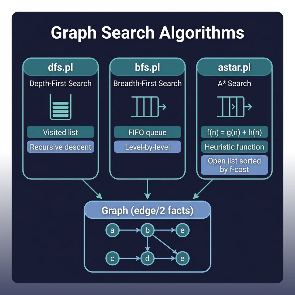
Depth-First and Breadth-First Search
With the graph loaded dynamically, the search modules simply import edge/2 from read_graph. Depth-first search explores as deep as possible along each branch before backtracking, using a visited list for cycle detection. Here is graph_search/prolog/dfs.pl:
 1 :- use_module(read_graph, [edge/2]).
 2
 3 %% dfs(+Start, +Goal, -Path)
 4 dfs(Start, Goal, Path) :-
 5     dfs(Start, Goal, [Start], Path).
 6
 7 dfs(Goal, Goal, Visited, Path) :-
 8     reverse(Visited, Path).
 9 dfs(Current, Goal, Visited, Path) :-
10     edge(Current, Next),
11     \+ member(Next, Visited),
12     dfs(Next, Goal, [Next|Visited], Path).
Breadth-first search instead explores all neighbors at the current depth before moving deeper, using an explicit queue of partial paths. Here is graph_search/prolog/bfs.pl:
 1 :- use_module(read_graph, [edge/2]).
 2
 3 %% bfs(+Start, +Goal, -Path)
 4 bfs(Start, Goal, Path) :-
 5     bfs_queue([[Start]], Goal, Path).
 6
 7 bfs_queue([[Goal|Visited]|_], Goal, Path) :-
 8     reverse([Goal|Visited], Path).
 9 bfs_queue([[Current|Visited]|Rest], Goal, Path) :-
10     findall(
11         [Next, Current|Visited],
12         (edge(Current, Next), \+ member(Next, [Current|Visited])),
13         Children
14     ),
15     append(Rest, Children, NewQueue),
16     bfs_queue(NewQueue, Goal, Path).
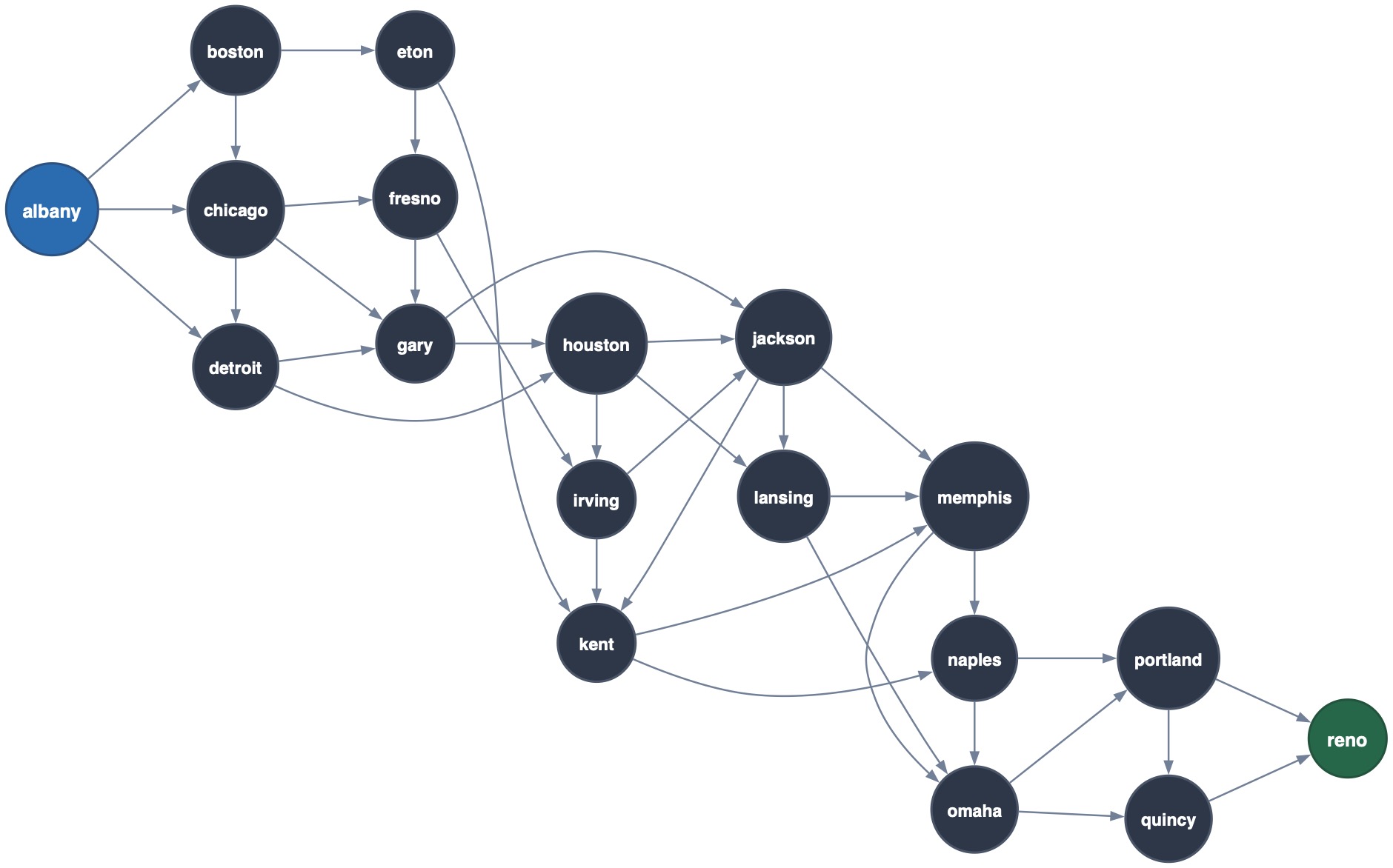
Running these on our 20-node city graph:
1 ?- dfs(albany, reno, Path).
2 Path = [albany, boston, chicago, detroit, gary, houston, irving, ...]
3
4 ?- bfs(albany, reno, Path).
5 Path = [albany, boston, eton, kent, naples, portland, reno]
Notice that BFS finds the shortest path (7 nodes), while DFS may explore a longer route through the interior of the graph.
Iterative Deepening
Depth-First Search (DFS) has a major space advantage: it only needs to store the path it is currently exploring, meaning its memory consumption is linear with the maximum depth of the search tree,  . However, DFS is not complete on infinite graphs and is not guaranteed to find the shortest path (as we saw on our city graph). Breadth-First Search (BFS) is complete and guarantees the shortest path, but its memory consumption is exponential,
  (where
  is the branching factor), because it must store all active paths in its queue.
Iterative Deepening Search (IDS) combines the best of both worlds: the space efficiency of DFS with the completeness and optimality of BFS.
IDS operates by repeatedly running a depth-limited DFS, starting with a depth limit of 1, and incrementing the limit on each iteration. Although it seems wasteful to re-explore the top parts of the search tree multiple times, the number of nodes at depth $d$ grows exponentially, so the overhead of re-exploring the shallower levels is minimal (usually under 11% for binary trees).
Custom Pure Prolog Implementation
In Prolog, we can implement IDS very elegantly. We use the built-in predicate between/3 to generate depth limits starting from 1, and then call a custom depth-limited DFS predicate:
 1 %% ids(+Start, +Goal, -Path)
 2 %% Iterative Deepening Search: increases depth limit incrementally.
 3 ids(Start, Goal, Path) :-
 4     between(1, 100, DepthLimit),
 5     depth_limited_dfs(Start, Goal, [Start], DepthLimit, Path).
 6
 7 %% depth_limited_dfs(+Current, +Goal, +Visited, +Limit, -Path)
 8 depth_limited_dfs(Goal, Goal, Visited, _, Path) :-
 9     !,
10     reverse(Visited, Path).
11 depth_limited_dfs(Current, Goal, Visited, Limit, Path) :-
12     Limit > 0,
13     edge(Current, Next),
14     \+ member(Next, Visited),
15     NextLimit is Limit - 1,
16     depth_limited_dfs(Next, Goal, [Next|Visited], NextLimit, Path).
Because of Prolog’s backtracking, if depth_limited_dfs/5 fails to find the goal within the current DepthLimit, Prolog backtracks to between/3, which increments DepthLimit to the next integer, and the search starts again with the larger limit. Like BFS, this guarantees that the first path found is the shortest path.
Built-in Support: call_with_depth_limit/3
SWI-Prolog also provides a built-in meta-predicate called call_with_depth_limit(:Goal, +Limit, -Result). This limits the depth of execution of any arbitrary Prolog goal (measured by the depth of the call stack).
If the goal succeeds within the limit, Result is unified with the number of stack frames used. If the limit is reached, Result unifies with the atom depth_limit_exceeded. We can use this to build a general-purpose iterative deepening search wrapper over our standard, unbounded dfs/3 predicate:
1 %% ids_builtin(+Start, +Goal, -Path)
2 ids_builtin(Start, Goal, Path) :-
3     between(1, 100, Limit),
4     call_with_depth_limit(dfs(Start, Goal, Path), Limit, Result),
5     Result \= depth_limit_exceeded.
This built-in approach is useful when you want to impose depth limits on complex reasoning rules or when wrapping existing code, though writing a custom depth_limited_dfs/5 predicate (as shown above) is usually preferred for finer search control.
A* Heuristic Search
A* combines the actual path cost with a heuristic estimate of the remaining distance to the goal. By maintaining an open list sorted by f-cost (g + h), it explores the most promising paths first. Here is graph_search/prolog/astar.pl:
 1 :- module(astar, [
 2     astar/4,
 3     distance_heuristic/2,
 4     zero_heuristic/2
 5 ]).
 6
 7 :- use_module(read_graph, [edge/2]).
 8
 9 %% Safe call: if Heuristic(Node, Value) fails with existence error,
10 %% return 0.
11 safe_call(Callable, Node, Value) :-
12     catch(call(Callable, Node, Value), _, Value = 0).
13
14 %% A* search: accepts both string designators ('h/2') and callable terms
15 %% (?(-N,-V)).
16 astar(Start, Goal, Heuristic, Path) :-
17     safe_call(Heuristic, Start, H0),
18     H is H0 + 0,
19     astar_loop([node(H, 0, [Start])], Goal, Heuristic, Path).
20
21 astar_loop([node(_, _, [Goal|Rest])|_], Goal, _, Path) :-
22     reverse([Goal|Rest], Path).
23 astar_loop([node(_, G, [Current|Rest])|Open], Goal, Heuristic, Path) :-
24     findall(
25         node(F1, G1, [Next, Current|Rest]),
26             (   edge(Current, Next),
27                 \+ member(Next, [Current|Rest]),
28             G1 is G + 1,
29             safe_call(Heuristic, Next, H0),
30             H is H0 + 0,
31             F1 is G1 + H
32             ),
33         Children
34        ),
35     append(Open, Children, Unsorted),
36     sort(1, @=<, Unsorted, Sorted),
37     astar_loop(Sorted, Goal, Heuristic, Path).
38
39 %% Zero heuristic: admissible for uniform-weight graphs (all edge
40 %% weights = 1).
41 %% Useful as a baseline for testing A* correctness.
42 zero_heuristic(_, 0).
43
44 %% Example heuristic: estimated remaining distance to goal (reno).
45 %% Rough estimates for the sample_graph cities — admissible for
46 %% uniform-weight graph.
47 distance_heuristic(reno,      0).
48 distance_heuristic(portland,  1).
49 distance_heuristic(quincy,    1).
50 distance_heuristic(omaha,     2).
51 distance_heuristic(naples,    2).
52 distance_heuristic(memphis,   3).
53 distance_heuristic(lansing,   3).
54 distance_heuristic(kent,      3).
55 distance_heuristic(jackson,   4).
56 distance_heuristic(irving,    4).
57 distance_heuristic(houston,   4).
58 distance_heuristic(gary,      5).
59 distance_heuristic(fresno,    5).
60 distance_heuristic(eton,      5).
61 distance_heuristic(detroit,   5).
62 distance_heuristic(chicago,   6).
63 distance_heuristic(boston,     6).
64 distance_heuristic(albany,    7).
1 ?- astar(albany, reno, distance_heuristic, Path).
2 Path = [albany, boston, eton, kent, naples, portland, reno]
The heuristic guides A* directly toward the goal, avoiding the unnecessary exploration of interior nodes that DFS would visit.
State-Space Search and Puzzle Solving
Many classic AI problems can be modeled as State-Space Search. In this paradigm, we define:
- State representation: A data structure representing the current configuration of the world (typically a Prolog compound term).
- Initial state: The starting configuration.
- Goal state: The target configuration we want to reach.
- State transitions (moves): Legal actions that transform one state into another.
- Constraints: Conditions that states must satisfy to be considered valid or safe.
Prolog is uniquely suited for state-space search because of its built-in backtracking and pattern matching. We can implement search algorithms (like DFS) to traverse the states automatically, and use unification to check if our current state matches the goal state.
The Farmer, Fox, Chicken, and Grain Puzzle
To illustrate, we solve the classic river crossing puzzle: a farmer must transport a fox, a chicken, and a sack of grain from the left bank of a river to the right bank. The constraints are:
- The farmer’s boat can only carry the farmer and at most one other item.
- If the farmer leaves the fox and chicken alone on a bank, the fox eats the chicken.
- If the farmer leaves the chicken and grain alone on a bank, the chicken eats the grain.
We represent the state as a compound term: state(Farmer, Fox, Chicken, Grain), where each argument can be either left or right to indicate which bank the item is currently on.
The puzzle_solver project implements this solver. Here is the complete file puzzle_solver/prolog/farmer.pl:
 1 %% farmer.pl - Farmer, Fox, Chicken, Grain river crossing puzzle
 2 %% Demonstrates state-space search with Prolog backtracking
 3 :- module(farmer, [
 4     solve_farmer/1
 5 ]).
 6
 7 %% State: state(Farmer, Fox, Chicken, Grain) where each is 'left' or
 8 %% 'right'
 9 %% Goal: all on the right bank
10
11 solve_farmer(Moves) :-
12     InitState = state(left, left, left, left),
13     GoalState = state(right, right, right, right),
14     solve(InitState, GoalState, [InitState], RevMoves),
15     reverse(RevMoves, Moves).
16
17 solve(Goal, Goal, _Visited, []).
18 solve(State, Goal, Visited, [Description|Moves]) :-
19     move(State, NextState, Description),
20     safe(NextState),
21     \+ member(NextState, Visited),
22     solve(NextState, Goal, [NextState|Visited], Moves).
23
24 %% Moves: farmer always crosses, optionally carrying one item
25 move(state(left,F,C,G), state(right,F,C,G), farmer_alone).
26 move(state(right,F,C,G), state(left,F,C,G), farmer_alone).
27 move(state(left,left,C,G), state(right,right,C,G), farmer_fox).
28 move(state(right,right,C,G), state(left,left,C,G), farmer_fox).
29 move(state(left,F,left,G), state(right,F,right,G), farmer_chicken).
30 move(state(right,F,right,G), state(left,F,left,G), farmer_chicken).
31 move(state(left,F,C,left), state(right,F,C,right), farmer_grain).
32 move(state(right,F,C,right), state(left,F,C,left), farmer_grain).
33
34 %% Safety: fox cannot be alone with chicken, chicken cannot be alone
35 %% with grain
36 safe(state(Farmer, Fox, Chicken, Grain)) :-
37     (Fox == Chicken -> Farmer == Fox ; true),
38     (Chicken == Grain -> Farmer == Chicken ; true).
Constraint-Based Search: The N-Queens Problem
A third powerful paradigm for search in Prolog is Constraint Logic Programming, specifically Constraint Logic Programming over Finite Domains (CLP(FD)). Instead of manually coding depth-first search or backtracking state transitions, you define variables, their domains, and the relationships (constraints) that must hold true. Prolog’s constraint solver then automatically propagates these constraints to prune the search space and find valid assignments.
To illustrate this, we can look at the classic N-Queens problem, which asks how to place  queens on an
  chessboard such that no two queens can attack each other. This means no two queens can share the same row, column, or diagonal.
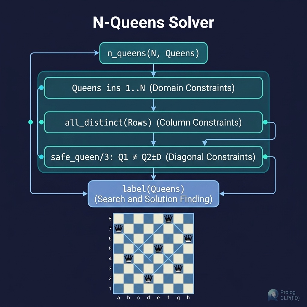
The companion project n_queens implements this solver. Here is the complete file n_queens/prolog/queens.pl:
 1 :- module(queens, [
 2     n_queens/2
 3 ]).
 4
 5 :- use_module(library(clpfd)).
 6
 7 %% n_queens(+N, -Queens)
 8 %% Queens is a list of column positions for queens in each row
 9 n_queens(N, Queens) :-
10     length(Queens, N),
11     Queens ins 1..N,
12     safe_queens(Queens),
13     label(Queens).
14
15 safe_queens([]).
16 safe_queens([Q|Qs]) :-
17     safe_queen(Q, Qs, 1),
18     safe_queens(Qs).
19
20 safe_queen(_, [], _).
21 safe_queen(Q, [Q1|Qs], D) :-
22     Q #\= Q1,
23     Q #\= Q1 + D,
24     Q #\= Q1 - D,
25     D1 #= D + 1,
26     safe_queen(Q, Qs, D1).
How the CLP(FD) Search Works
- Representation: We represent the board as a list of length called
Queens. The index of an element in the list represents the row number (1 to), and the value at that index represents the column number of the queen in that row.
- Domain:
Queens ins 1..Nestablishes that each variable in theQueenslist must be an integer between and .
and .
- Column Constraints: Since each row has exactly one queen, we only need to ensure no two queens share a column. By using the list representation, the index ensures row uniqueness. The column constraint
Q #\= Q1(insafe_queen/3) ensures that no two queens share the same column. -
Diagonal Constraints: Two queens at columns
 and
and  separated by
  rows are on the same diagonal if
  . This is elegantly modeled using two inequality constraints:
Q #\= Q1 + D(upper-diagonal check)Q #\= Q1 - D(lower-diagonal check)
- Labeling:
label(Queens)tells the constraint solver to perform the backtracking search to assign concrete values to the variables in theQueenslist that satisfy all constraints.
Running the Solver
You can run queries in the REPL to solve for a specific size :
1 ?- n_queens(8, Queens).
2 Queens = [1, 5, 8, 6, 3, 7, 2, 4] .
To count the total number of solutions for an 8x8 board:
1 ?- aggregate_all(count, n_queens(8, _), Count).
2 Count = 92.
CLP(FD) propagation dramatically prunes the search space relative to a naive backtracking search, making the search for solutions extremely efficient even for larger board sizes.
Optional Practice Problems
- Weighted Graph Search: In the
graph_searchproject, modify the graph definition to include edge weights. Then implement a uniform-cost search (or Dijkstra’s algorithm) to find the shortest path between two nodes in terms of cumulative edge weights. - Farmer Puzzle Variation: In the
puzzle_solverproject, adapt thefarmer.plrules to allow the boat to hold the farmer and up to two items, but add a new constraint that the wolf and the goat cannot be left alone on either bank, nor can the goat and the cabbage.