Reasoning and Inference

Prolog is fundamentally a reasoning engine. In this chapter we explore how to use Prolog for various forms of logical reasoning that are central to AI.

Propositional and First-Order Logic in Prolog

Prolog predicates naturally map to First-Order Logic (FOL). We express propositional variables as simple arity-0 facts, and relational predicates with variables to represent quantified logical statements.

Horn Clauses

Classical logic allows rules with arbitrary conjunctions, disjunctions, and negations. However, resolving arbitrary first-order formulas is computationally expensive. To remain efficient, Prolog restricts its database to Horn clauses.

A Horn clause is a disjunction of literals with at most one positive (non-negated) literal. In classical notation:

A \lor \neg B_1 \lor \neg B_2 \lor \dots \lor \neg B_n

By applying Boolean algebra, this is logically equivalent to the implication:

(B_1 \land B_2 \land \dots \land B_n) \Rightarrow A

In Prolog, this implication is written in reverse as:

1 A :- B1, B2, ..., Bn.

A is the head (positive literal).
B1, B2, ..., Bn make up the body (conjunctive negative literals).
If there is no body, the clause is a fact (equivalent to a positive literal asserting truth).
If there is no head, the clause represents a query (a goal to be disproven via contradiction).

Mapping Logic to Prolog

While this Horn clause format is highly efficient for execution using SLD Resolution, it does place some limitations on what can be directly expressed:

Universal Quantifiers (\forall$): Implicitly assumed for all variables in a rule.
Existential Quantifiers (\exists$): Represented by introducing new variables on the right-hand side of a rule (e.g. has_child(X) :- parent(X, _). means “For all X, X has a child if there exists some Y such that X is a parent of Y”).
Disjunction in the Head: Prolog does not allow disjunctive heads like A or B :- C.. You must split this into multiple rules, or use helper predicates.

Figure 7. Architecture diagram for the Inference Engine example

Forward and Backward Chaining

In logic systems, we use two main strategies to apply rules to facts:

Backward Chaining (Goal-Driven)

Backward chaining starts with a goal (query) and works backward, matching it against rule heads to find the subgoals (body conditions) needed to prove it. This recursion continues until all subgoals are resolved by direct facts in the database.

Prolog’s Default: This is Prolog’s built-in execution strategy.
When to Use: Best when you have a specific goal to prove and a large number of facts, but only a small subset are relevant to the query.

Forward Chaining (Data-Driven)

Forward chaining starts with known facts and applies rules to derive new facts. These new facts are asserted into the database, and the process repeats until a fixpoint is reached (i.e., no more new facts can be derived).

When to Use: Best when you want to discover everything that follows from a set of starting data, such as in configuration systems, event monitors, or scheduling pipelines.

Here is a comparison of the two approaches:

Feature	Backward Chaining	Forward Chaining
Direction	Goal `\to`$ Facts	Facts `\to`$ Conclusions
Prolog Integration	Native execution engine	Needs custom meta-interpreter
Space Complexity	Low (only stores active path in stack)	High (asserts all derived facts on heap)
Best Fit	Diagnostic queries, verification	Event monitoring, data analysis

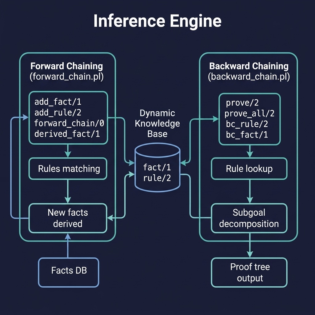
The inference_engine project implements a forward-chaining engine that derives new facts from rules until a fixpoint is reached. Here is the file inference_engine/prolog/forward_chain.pl:

 1 %% forward_chain.pl - Forward chaining inference engine
 2 %% Derives new facts from rules until no more can be derived
 3 :- module(forward_chain, [
 4     forward_chain/0,
 5     add_rule/2,
 6     add_fact/1,
 7     derived_fact/1
 8 ]).
 9 
10 :- dynamic fact/1.
11 :- dynamic rule/2.
12 
13 %% add_fact(+Fact) - Assert a new fact
14 add_fact(F) :- \+ fact(F), assert(fact(F)).
15 add_fact(_).
16 
17 %% add_rule(+Conditions, +Conclusion)
18 add_rule(Conditions, Conclusion) :-
19     assert(rule(Conditions, Conclusion)).
20 
21 %% derived_fact(?F) - Query derived facts
22 derived_fact(F) :- fact(F).
23 
24 %% forward_chain - Apply all rules until fixpoint
25 forward_chain :-
26     rule(Conditions, Conclusion),
27     \+ fact(Conclusion),
28     all_conditions_met(Conditions),
29     assert(fact(Conclusion)),
30     !,
31     forward_chain.
32 forward_chain. % fixpoint reached
33 
34 all_conditions_met([]).
35 all_conditions_met([C|Rest]) :-
36     fact(C),
37     all_conditions_met(Rest).

And a backward-chaining engine with explanation traces. Here is the file inference_engine/prolog/backward_chain.pl:

 1 :- module(backward_chain, [
 2     prove/2
 3 ]).
 4 
 5 :- dynamic bc_rule/2.
 6 :- dynamic bc_fact/1.
 7 
 8 %% prove(+Goal, -Proof) - Prove a goal and return the proof tree
 9 prove(Goal, fact(Goal)) :-
10     bc_fact(Goal).
11 prove(Goal, rule(Goal, Proofs)) :-
12     bc_rule(Conditions, Goal),
13     prove_all(Conditions, Proofs).
14 
15 prove_all([], []).
16 prove_all([C|Rest], [P|Proofs]) :-
17     prove(C, P),
18     prove_all(Rest, Proofs).

Generating and Visualizing Proof Trees

While deriving conclusions is useful, in many AI applications (such as expert systems) we must also explain why a conclusion was reached. A proof tree is a tree-like data structure that records the steps, rules, and facts used to satisfy a goal.

Prolog is well-suited for building proof trees because we can easily write a meta-interpreter—a Prolog program that reads and executes other Prolog programs.

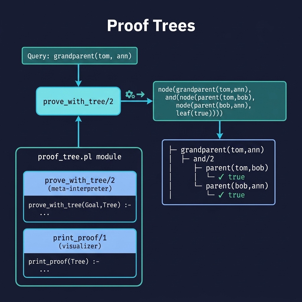
Figure 8. Architecture diagram for the Proof Trees example

The companion project proof_trees demonstrates this technique. Here is the core file proof_trees/prolog/proof_tree.pl:

 1 %% proof_tree.pl - Build and display proof trees
 2 %% for explainable reasoning
 3 :- module(proof_tree, [
 4     prove_with_tree/2,
 5     print_proof/1,
 6     sample_data_loaded/0
 7 ]).
 8 
 9 sample_data_loaded :-
10     (   exists_file('sample_data.pl')
11     ->  consult('sample_data.pl')
12     ;   exists_file('prolog/sample_data.pl')
13     ->  consult('prolog/sample_data.pl')
14     ;   format(user_error, 'WARNING: sample_data.pl not found~n', []),
15         fail
16     ).
17 
18 :- initialization(sample_data_loaded).
19 
20 %% prove_with_tree(+Goal, -Tree) - Prove and return proof tree
21 prove_with_tree(true, leaf(true)) :- !.
22 prove_with_tree((A, B), and(PA, PB)) :- !,
23     prove_with_tree(A, PA),
24     prove_with_tree(B, PB).
25 %% Handle negation-as-failure (meta-builtin)
26 prove_with_tree(\+ G, node(\+ G, leaf(\+ G))) :- !,
27     \+ G.
28 %% Handle not-unifiable (builtin comparison)
29 prove_with_tree(X \= Y, node(X\=Y, leaf(X\=Y))) :- !,
30     X \= Y.
31 %% User-defined goals: look up clauses and recurse
32 prove_with_tree(Goal, node(Goal, ChildProofs)) :-
33     clause(Goal, Body),
34     prove_with_tree(Body, ChildProofs).
35 
36 %% print_proof(+Tree) - Pretty-print a proof tree with indentation
37 print_proof(Tree) :- print_proof(Tree, 0).
38 
39 print_proof(leaf(true), Indent) :- !,
40     tab(Indent), format("✓ true~n").
41 print_proof(leaf(Goal), Indent) :-
42     tab(Indent), format("✓ ~w~n", [Goal]).
43 print_proof(and(A, B), Indent) :-
44     print_proof(A, Indent),
45     print_proof(B, Indent).
46 print_proof(node(Goal, Children), Indent) :-
47     tab(Indent), format("├─ ~w~n", [Goal]),
48     Indent1 is Indent + 3,
49     print_proof(Children, Indent1).

How the Meta-Interpreter Works

Base Cases: When the goal is true, it is trivially proven and returns leaf(true).
Conjunctions: For a goal composed of (A, B), it recursively proves A (producing proof tree PA) and B (producing PB), and returns and(PA, PB).
Built-in Handling: Special handlers are defined for negation-as-failure (\+ G) and inequality checks (X \= Y).
Clause Inspection: For user-defined predicates, clause(Goal, Body) is a built-in Prolog feature that inspects the database, finding a rule whose head matches Goal and returning its Body. The interpreter then recurses on the Body to find child proofs.

Running the Proof Visualizer

If we query the sample family relationships database:

1 ?- prove_with_tree(grandparent(adam, mary), Tree), print_proof(Tree).
2 ├─ grandparent(adam, mary)
3    ├─ parent(adam, john)
4       ✓ true
5    ├─ parent(john, mary)
6       ✓ true

This gives us a readable, tree-structured explanation of the system’s reasoning process.

 1 ## Reasoning with Uncertainty
 2 
 3 In real-world applications, reasoning is rarely black-and-white. AI systems must often handle uncertain or probabilistic information. One classic approach to this is attaching **certainty factors** or probabilities to rules and facts, and propagating those scores through the inference chain.
 4 
 5 To compute the probability of a derived goal, we apply the rules of probability:
 6 1. **Conjunction (AND)**: If a rule depends on multiple conditions, the probability of the conditions holding jointly is the product of their individual probabilities (assuming independence):
 7    {$$}
 8    P(A \land B) = P(A) \times P(B)
 9    {/$$}
10 2. **Rule Application**: The probability of the conclusion is the joint probability of its conditions multiplied by the conditional probability (confidence) of the rule:
11    {$$}
12    P(Conclusion) = P(Conditions) \times P(Rule)
13    {/$$}
14 
15 The companion project **prob_reasoning** implements this logic. Here is the complete file **prob_reasoning/prolog/prob_facts.pl**:
16 
17 ```prolog
18 %% prob_facts.pl - Probabilistic reasoning with certainty factors
19 :- module(prob_facts, [
20     prob_fact/2,
21     prob_rule/3,
22     prob_query/2
23 ]).
24 
25 :- dynamic prob_fact/2.  % prob_fact(Fact, Probability)
26 :- dynamic prob_rule/3;  % prob_rule(Conditions, Conclusion, CondProb)
27 
28 %% prob_query(+Goal, -Probability)
29 %% Query the probability of a goal given known facts and rules
30 prob_query(Goal, Prob) :-
31     prob_fact(Goal, Prob), !.
32 prob_query(Goal, Prob) :-
33     prob_rule(Conditions, Goal, CondProb),
34     maplist(prob_query, Conditions, CondProbs),
35     foldl(mul, CondProbs, 1.0, JointProb),
36     Prob is JointProb * CondProb.
37 
38 mul(X, Acc, Result) :- Result is Acc * X.

If we query the weather database defined in this project:

1 ?- prob_query(storm, Prob).
2 Prob = 0.105.

 1 ## Abductive Reasoning
 2 
 3 Abductive reasoning is the process of reasoning from **observations** to the most likely **explanations** (or hypotheses) that could cause them. It is often described as "inference to the best explanation."
 4 - **Deduction**: Given `A`$ and `A \Rightarrow B`$, derive `B`$.
 5 - **Induction**: Given examples of `A`$ and `B`$, derive the rule `A \Rightarrow B`$.
 6 - **Abduction**: Given `B`$ and `A \Rightarrow B`$, hypothesize `A`$ as the explanation for `B`$.
 7 
 8 In Prolog, we can implement abductive reasoning by defining a set of **abducible predicates**—facts that we are allowed to assume true if they help explain the observation.
 9 
10 Here is a simple abductive meta-interpreter:
11 
12 ```prolog
13 %% abduce(+Goal, +Abducibles, -Explanation)
14 %% Finds a set of abducible assumptions that prove Goal
15 abduce(true, _, []) :- !.
16 abduce((A, B), Abducibles, Expl) :- !,
17     abduce(A, Abducibles, ExplA),
18     abduce(B, Abducibles, ExplB),
19     append(ExplA, ExplB, Expl).
20 abduce(Goal, Abducibles, [Goal]) :-
21     member(Goal, Abducibles).
22 abduce(Goal, Abducibles, Expl) :-
23     clause(Goal, Body),
24     abduce(Body, Abducibles, Expl).

If we define the rules:

1 grass_is_wet :- rained.
2 grass_is_wet :- sprinkler_was_on.

And declare [rained, sprinkler_was_on] as our list of abducibles, calling abduce(grass_is_wet, [rained, sprinkler_was_on], Expl) will backtrack to yield two possible explanations: [rained] or [sprinkler_was_on].

Non-Monotonic Reasoning and Defaults

Classical logic is monotonic: once a conclusion is proven true, adding new facts to the database can never invalidate it. However, human reasoning is often non-monotonic: we draw default conclusions that we retract when we receive new, contradictory information.

Prolog implements non-monotonic reasoning using the Closed-World Assumption and Negation as Failure (\+). We can write default rules that hold true unless an exception is proven.

Default Logic Example

A classic example is reasoning about bird flight: “Birds fly by default, unless they are abnormal (like penguins or ostriches).”

 1 flies(X) :-
 2     bird(X),
 3     \+ abnormal(X).
 4 
 5 abnormal(X) :- penguin(X).
 6 abnormal(X) :- ostrich(X).
 7 
 8 bird(tweety).
 9 bird(pingu).
10 penguin(pingu).

If we query the database:

?- flies(tweety). succeeds because bird(tweety) is true and abnormal(tweety) cannot be proven (fails).
?- flies(pingu). fails because penguin(pingu) is asserted, which proves abnormal(pingu), thereby causing \+ abnormal(pingu) to fail.

If we later learn that Tweety is actually a penguin and assert penguin(tweety)., the previous conclusion flies(tweety) is automatically retracted—demonstrating non-monotonic behavior.

Case Study: A Medical Diagnosis Reasoner

To see how these reasoning techniques come together, we can look at a practical case study: a Medical Diagnosis Reasoner. This system diagnoses diseases by matching patient symptoms against a clinical knowledge base and generating an explicit explanation.

The companion project medical_diagnosis implements this diagnostic reasoner. The program uses a clean rule-matching approach:

It accepts a list of patient symptoms and asserts them dynamically into the database.
It queries the disease knowledge base to find a disease whose required symptoms are a subset of the patient’s symptoms.
It formats a diagnostic explanation.
It cleans up the temporary asserted facts to prevent side effects in subsequent runs.

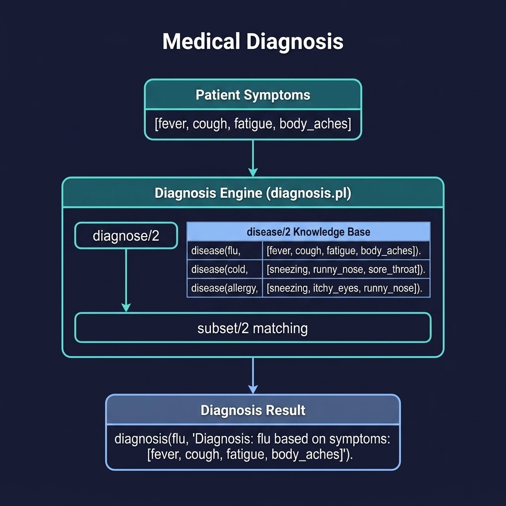
Figure 9. Architecture diagram for the Medical Diagnosis example

The medical_diagnosis project demonstrates rule-based diagnostic reasoning. Here is the file medical_diagnosis/prolog/diagnosis.pl:

 1 :- module(diagnosis, [
 2     diagnose/2,
 3     symptom/1
 4 ]).
 5 
 6 :- dynamic symptom/1.
 7 
 8 %% diagnose(+PatientSymptoms, -DiagnosisWithExplanation)
 9 diagnose(Symptoms, diagnosis(Disease, Explanation)) :-
10     maplist(assert_symptom, Symptoms),
11     disease(Disease, RequiredSymptoms),
12     subset(RequiredSymptoms, Symptoms),
13     format(atom(Explanation),
14            'Diagnosis: ~w based on symptoms: ~w',
15            [Disease, RequiredSymptoms]),
16     retract_symptoms(Symptoms).
17 
18 assert_symptom(S) :- assert(symptom(S)).
19 retract_symptoms([]).
20 retract_symptoms([S|Rest]) :- retract(symptom(S)),
21     retract_symptoms(Rest).
22 
23 %% Disease knowledge base
24 disease(flu, [fever, cough, fatigue, body_aches]).
25 disease(cold, [sneezing, runny_nose, sore_throat]).
26 disease(allergy, [sneezing, itchy_eyes, runny_nose]).
27 disease(bronchitis, [cough, chest_pain, fatigue, shortness_of_breath]).
28 disease(migraine, [headache, nausea, light_sensitivity]).

Here is sample output:

TBD

Up next

Expert Systems and Rule-Based AI