Meta-Interpreters: Prolog Reasoning About Prolog

Meta-interpreters are one of Prolog’s most unique and powerful capabilities. A meta-interpreter is a Prolog program that interprets Prolog programs, allowing us to modify, extend, or instrument the reasoning process itself. This is a form of computational reflection: the language turns its inference engine inward, treating its own rules and facts as data to be examined, transformed, and re-executed under new policies.

Why does this matter? In most programming languages, if you want to change how code executes (to add tracing, limit recursion depth, try alternative search strategies, or attach uncertainty scores to conclusions), you modify the compiler or runtime, write a DSL, or build an external tool. In Prolog, you write a half-dozen lines of Prolog. The meta-interpreter sits above the base language yet within it, intercepting every resolution step and deciding what to do next. This makes Prolog uniquely suited to tasks like explainable AI, automated debugging, and reasoning under resource constraints.

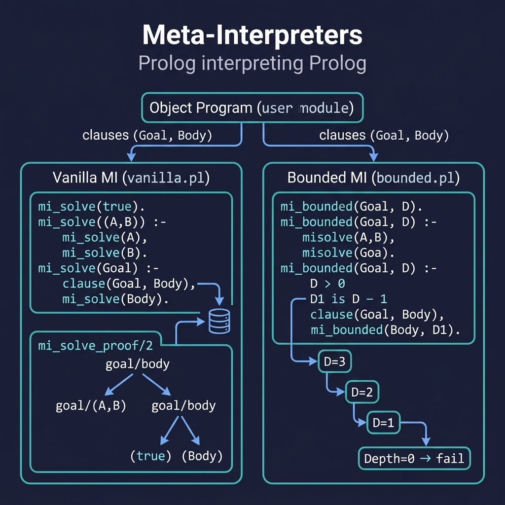
The simplest meta-interpreter — sometimes called the “vanilla” meta-interpreter — is a Prolog interpreter written in Prolog. Despite its brevity, it faithfully mirrors Prolog’s own execution model: depth-first search with backtracking, left-to-right subgoal ordering, and resolution via clause lookup.

The key built-in predicate is clause(Head, Body), which retrieves the clauses of a predicate from the program database. Given a goal term Head, clause/2 nondeterministically returns each matching clause, binding Body to the clause body (or true if it’s a fact). On backtracking, it returns the next clause. This is the reflective mechanism that lets a meta-interpreter “see” the program it’s interpreting.

The vanilla meta-interpreter uses exactly three clauses, corresponding to the three kinds of goals Prolog encounters:

1. The goal true: always succeeds. The meta-interpreter handles this as a base case with a cut to prevent backtracking into other clauses.

2. A conjunction (A, B): the meta-interpreter decomposes it, solving A first (which may bind variables), then solving B in the resulting environment. The cut ensures this is recognized before the general goal clause.

3. Any other goal: the meta-interpreter looks up matching clauses with clause/2. For each matching clause body, it recursively interprets the body. If no clauses match, the goal simply fails; if multiple clauses match, Prolog’s native backtracking explores each in turn.

This three-clause structure is the template from which all other meta-interpreters are derived. Every extension we build (proof trees, depth bounds, uncertainty propagation, custom search) starts by modifying one or more of these clauses.

The meta_interp project provides both a vanilla and bounded meta-interpreter. Here is the file meta_interp/prolog/vanilla.pl:

 1 :- module(vanilla, [
 2     mi_solve/1,
 3     mi_solve/2,
 4     mi_solve_proof/2,
 5     mi_solve_proof/3
 6 ]).
 7 
 8 %% mi_solve(+Goal) - Vanilla meta-interpreter (user module context)
 9 mi_solve(Goal) :- mi_solve(user, Goal).
10 
11 %% mi_solve(+Module, +Goal)
12 %% Vanilla meta-interpreter with module context
13 mi_solve(_, true) :- !.
14 mi_solve(Mod, (A, B)) :- !, mi_solve(Mod, A), mi_solve(Mod, B).
15 mi_solve(Mod, Goal) :-
16     clause(Mod:Goal, Body),
17     mi_solve(Mod, Body).
18 
19 %% mi_solve_proof(+Goal, -Proof)
20 %% Meta-interpreter with proof tree (user module)
21 mi_solve_proof(Goal, Proof) :- mi_solve_proof(user, Goal, Proof).
22 
23 %% mi_solve_proof(+Module, +Goal, -Proof) - With module context
24 mi_solve_proof(_, true, true) :- !.
25 mi_solve_proof(Mod, (A, B), (PA, PB)) :- !,
26     mi_solve_proof(Mod, A, PA),
27     mi_solve_proof(Mod, B, PB).
28 mi_solve_proof(Mod, Goal, Goal-Proof) :-

Notice the module-aware variants (mi_solve/2 and mi_solve_proof/3). By qualifying the clause/2 lookup with a module prefix (Mod:Goal), the meta-interpreter can operate over predicates defined in any module, not just the one it’s loaded into. This is essential for building reusable reasoning tools that work across different knowledge bases. The proof-tree variant (mi_solve_proof) returns a nested term rather than just succeeding or failing: a preview of the explanation capabilities we’ll explore next.

A meta-interpreter that merely succeeds or fails tells us whether a conclusion follows from our knowledge base, but not why. For explainable AI where a system must justify its reasoning to a user, an auditor, or another system, we need to capture the inference path. This is where proof trees come in.

A proof tree is a data structure that records every resolution step the meta-interpreter takes: which goal was proved, which clause was used, and what sub-proofs were required. It transforms the meta-interpreter from a yes/no oracle into a transparent reasoner.

The proof_trees project provides a standalone proof tree builder with its own rich sample dataset. Rather than requiring users to assert facts manually, the module auto-loads a comprehensive 5-generation family tree from prolog/sample_data.pl, containing 28 parent facts and 7 derived relationship predicates:

Here is the updated proof_trees/prolog/proof_tree.pl:

 1 :- module(proof_tree, [
 2     prove_with_tree/2,
 3     print_proof/1,
 4     sample_data_loaded/0
 5 ]).
 6 
 7 %% Load sample data - try multiple paths for
 8 %% different working directories
 9 sample_data_loaded :-
10     (   exists_file('sample_data.pl')
11     ->  consult('sample_data.pl')
12     ;   exists_file('prolog/sample_data.pl')
13     ->  consult('prolog/sample_data.pl')
14     ;   format(user_error, 'WARNING: sample_data.pl not found~n', []),
15         fail
16     ).
17 
18 :- initialization(sample_data_loaded).
19 
20 %% prove_with_tree(+Goal, -Tree) - Prove and return proof tree
21 prove_with_tree(true, leaf(true)) :- !.
22 prove_with_tree((A, B), and(PA, PB)) :- !,
23     prove_with_tree(A, PA),
24     prove_with_tree(B, PB).
25 %% Handle negation-as-failure (meta-builtin)
26 prove_with_tree(\+ G, node(\+ G, leaf(\+ G))) :- !,
27     \+ G.
28 %% Handle not-unifiable (builtin comparison)
29 prove_with_tree(X \= Y, node(X\=Y, leaf(X\=Y))) :- !,
30     X \= Y.
31 %% User-defined goals: look up clauses and recurse
32 prove_with_tree(Goal, node(Goal, ChildProofs)) :-
33     clause(Goal, Body),
34     prove_with_tree(Body, ChildProofs).
35 
36 %% print_proof(+Tree) - Pretty-print a proof tree with indentation
37 print_proof(Tree) :- print_proof(Tree, 0).
38 
39 print_proof(leaf(true), Indent) :- !,
40     tab(Indent), format("✓ true~n").
41 print_proof(leaf(Goal), Indent) :-
42     tab(Indent), format("✓ ~w~n", [Goal]).
43 print_proof(and(A, B), Indent) :-
44     print_proof(A, Indent),
45     print_proof(B, Indent).
46 print_proof(node(Goal, Children), Indent) :-

One subtlety that emerges when building proof trees is the treatment of built-in predicates. When prove_with_tree encounters a goal like X \= Y or \+ sibling(X, Y), it cannot use clause/2 to look up a body — these are system predicates with no user-accessible clause definitions. Attempting clause/2 on a built-in raises a permission error. The original proof tree code handled only user-defined goals and true, which worked for simple examples but broke as soon as predicates like sibling/2 (which uses \=) or cousin/2 (which uses \+) appeared.

The updated version adds explicit clauses for \+/1 (negation-as-failure) and \=/2 (not unifiable). Each is treated as a leaf node in the tree, with the built-in executed directly via call/1. The leaf carries the original goal term — so when pretty-printed, you see entries like ✓ ann\=bob and ✓ \+sibling(carol,emma), making the reasoning steps visible even though they don’t decompose further.

Let’s examine actual proof tree output from the extended sample data. Each example illustrates a different reasoning pattern:

Direct fact lookup is the simplest possible proof:

1 ├─ parent(adam,john)
2    ✓ true

A single clause lookup finds parent(adam, john) as a fact (body true), producing a one-level tree.

Conjunction — grandparent(john, ann) requires proving two subgoals:

1 ├─ grandparent(john,ann)
2    ├─ parent(john,mary)
3       ✓ true
4    ├─ parent(mary,ann)
5       ✓ true

The meta-interpreter decomposes the conjunction into parent(john, mary) and parent(mary, ann), proving each independently. The tree structure mirrors the logical structure of the rule grandparent(X, Z) :- parent(X, Y), parent(Y, Z).

Recursive descent — a 5-generation ancestor chain from Adam to Grace:

 1 ├─ ancestor(adam,grace)
 2    ├─ parent(adam,john)
 3       ✓ true
 4    ├─ ancestor(john,grace)
 5       ├─ parent(john,mary)
 6          ✓ true
 7       ├─ ancestor(mary,grace)
 8          ├─ parent(mary,ann)
 9             ✓ true
10          ├─ ancestor(ann,grace)
11             ├─ parent(ann,carol)
12                ✓ true
13             ├─ ancestor(carol,grace)
14                ├─ parent(carol,grace)
15                   ✓ true

This tree traces the lineage adam → john → mary → ann → carol → grace. Each level of recursion adds a parent/2 leaf and a recursive ancestor/2 subgoal, until the base case (parent(carol, grace)) terminates the chain. The indentation makes the depth of the inference immediately visible — a 5-generation chain produces a 9-line proof tree.

Built-in comparison — sibling(ann, bob) incorporates an inequality check:

1 ├─ sibling(ann,bob)
2    ├─ parent(mary,ann)
3       ✓ true
4    ├─ parent(mary,bob)
5       ✓ true
6    ├─ ann\=bob
7       ✓ ann\=bob

The final subgoal ann \= bob is printed as a leaf showing the built-in comparison. Without this check, the sibling rule would also report that Ann is her own sibling (since parent(mary, ann) and parent(mary, ann) would both succeed).

Negation-as-failure like cousin(carol, emma) uses \+ sibling(carol, emma):

 1 ├─ cousin(carol,emma)
 2    ├─ grandparent(mary,carol)
 3       ├─ parent(mary,ann)
 4          ✓ true
 5       ├─ parent(ann,carol)
 6          ✓ true
 7    ├─ grandparent(mary,emma)
 8       ├─ parent(mary,bob)
 9          ✓ true
10       ├─ parent(bob,emma)
11          ✓ true
12    ├─ carol\=emma
13       ✓ carol\=emma
14    ├─ \+sibling(carol,emma)
15       ✓ \+sibling(carol,emma)

Carol and Emma share grandmother Mary, making them cousins but they could also have been siblings if they shared a parent. The \+ sibling/2 goal confirms they aren’t, and the proof tree records this check as a visible leaf node. (Note: this query actually has two solutions; Mary and Tom are both grandparents of both children so backtracking would produce a second tree with grandparent(tom, ...) variants.)

Derived predicates like aunt_uncle(michael, ann) chains two relationships:

 1 ├─ aunt_uncle(michael,ann)
 2    ├─ parent(mary,ann)
 3       ✓ true
 4    ├─ sibling(michael,mary)
 5       ├─ parent(john,michael)
 6          ✓ true
 7       ├─ parent(john,mary)
 8          ✓ true
 9       ├─ michael\=mary
10          ✓ michael\=mary

Michael is Ann’s uncle because he is a sibling of Ann’s parent Mary (they share father John). The proof tree shows the two-stage derivation: first establish that Mary is Ann’s parent, then prove that Michael and Mary are siblings.

Inverse relationships — descendant(grace, adam) uses ancestor/2 in reverse:

 1 ├─ descendant(grace,adam)
 2    ├─ ancestor(adam,grace)
 3       ├─ parent(adam,john)
 4          ✓ true
 5       ├─ ancestor(john,grace)
 6          ├─ parent(john,mary)
 7             ✓ true
 8          ├─ ancestor(mary,grace)
 9             ├─ parent(mary,ann)
10                ✓ true
11             ├─ ancestor(ann,grace)
12                ├─ parent(ann,carol)
13                   ✓ true
14                ├─ ancestor(carol,grace)
15                   ├─ parent(carol,grace)
16                      ✓ true

This tree reveals the full 6-generation path from Adam down to Grace. The descendant/2 rule is a single clause: descendant(X, Y) :- ancestor(Y, X). The proof tree captures the entire ancestor chain that justifies the descendant relationship.

Proof trees bridge the gap between logical inference and human-understandable explanation. In expert systems, they let a domain expert verify that the system’s conclusions follow from the intended rules. In legal or regulatory applications, they provide an audit trail. In interactive AI assistants, they let users ask “why did you conclude that?” and receive a structured answer. The proof tree is not a post-hoc rationalization stitched on after the fact because it is the reasoning, captured as it happens by a meta-interpreter that observes every step of its own execution.

Prolog’s native depth-first search has a well-known vulnerability: if a predicate can generate an infinite chain of subgoals, either through a buggy recursive rule or through cyclic data, the interpreter will descend forever, eventually exhausting the stack. In open-world settings like the semantic web or knowledge graphs constructed from crawled data, cycles are not bugs they’re facts of life. An employee works for a division, which belongs to a company, which owns a subsidiary, which employs the same person. Unchecked recursion over such data is a guaranteed infinite loop.

The bounded meta-interpreter solves this by adding a depth counter that decrements with each resolution step. When the counter reaches zero, the current branch of the search tree is pruned. This is not a heuristic, it is a guarantee of termination. For any knowledge base and any query, mi_bounded(Goal, MaxDepth) will either succeed or fail in finite time.

Here is the file meta_interp/prolog/bounded.pl:

 1 :- module(bounded, [
 2     mi_bounded/2,
 3     mi_bounded/3
 4 ]).
 5 
 6 %% mi_bounded(+Goal, +MaxDepth) - Solve with depth limit (user module)
 7 mi_bounded(Goal, MaxDepth) :- mi_bounded(user, Goal, MaxDepth).
 8 
 9 %% mi_bounded(+Module, +Goal, +MaxDepth)
10 %% Solve with depth limit and module context
11 mi_bounded(_, true, _) :- !.
12 mi_bounded(_, _, D) :- D =< 0, !, fail.
13 mi_bounded(Mod, (A, B), D) :- !,
14     mi_bounded(Mod, A, D),
15     mi_bounded(Mod, B, D).
16 mi_bounded(Mod, Goal, D) :-
17     D > 0,
18     clause(Mod:Goal, Body),

The depth limit operates on the inference depth, not the recursion depth of a single predicate. If a goal requires three levels of clause resolution to prove, say, grandparent(X, Z) → parent(X, Y) → parent(Y, Z) → true, that consumes three depth units. The same limit applies regardless of which predicates are involved: a shallow chain through many different predicates and a deep chain through a single recursive predicate are both bounded by the same MaxDepth.

This has practical implications. A depth of 1 means only facts can be proved — no rules are allowed to fire. A depth of 2 allows rules whose bodies contain only facts. Each increment of the depth bound enables one more “hop” through the inference graph. For applications like knowledge graph traversal, you might set MaxDepth to the maximum path length you’re willing to consider, effectively implementing a bounded path query in three lines of meta-interpreter code.

Iterative deepening: running the bounded meta-interpreter with successively larger depth limits is a standard technique for finding the “shallowest” proof first. Start with MaxDepth = 1, then 2, then 3, and so on. The first solution found is guaranteed to have the minimum inference depth. This combines the completeness of breadth-first search with the space efficiency of depth-first search, and it’s implemented entirely in the calling code, not in the meta-interpreter itself.

Classical logic programming operates in a binary world: a proposition is either proved or not. But many real-world reasoning tasks require gradations of belief. A medical diagnosis system shouldn’t just say “the patient has condition X;” it should attach a likelihood. A fraud detection system should report confidence scores, not boolean flags. A recommender system should rank suggestions by strength of evidence.

Meta-interpreters give us a clean way to add uncertainty reasoning without modifying the underlying knowledge base. The key insight: certainty factors, probabilities, or fuzzy truth values can be propagated through the proof tree in parallel with logical inference. The meta-interpreter proves a goal and simultaneously computes a combined certainty score from the scores of the sub-proofs.

Consider a certainty-factor approach. Each clause is annotated with a certainty factor between 0.0 (no confidence) and 1.0 (certain). Facts have direct certainty values; rules combine the certainties of their subgoals. The meta-interpreter pattern would look like:

 1 %% Conceptual sketch — not part of the companion code
 2 mi_certain(_, true, 1.0) :- !.
 3 mi_certain(Mod, (A, B), CF) :- !,
 4     mi_certain(Mod, A, CF1),
 5     mi_certain(Mod, B, CF2),
 6     CF is min(CF1, CF2).              % Conjunction: weakest link
 7 mi_certain(Mod, Goal, CF) :-
 8     clause_cf(Mod:Goal, Body, RuleCF),
 9     mi_certain(Mod, Body, BodyCF),
10     CF is RuleCF * BodyCF.            % Combine rule certainty with body proof

The conjunction case uses min because a chain of reasoning is only as strong as its weakest link. The goal case multiplies the rule’s own certainty factor by the combined certainty of its body. Different combination functions model different uncertainty calculi: fuzzy logic uses min and max, probability theory uses multiplication with independence assumptions, Dempster-Shafer theory uses belief and plausibility intervals.

What makes this powerful is the separation of concerns. The domain expert writes ordinary Prolog rules describing what is true. A separate annotation layer adds how certain each rule is. The meta-interpreter weaves them together at query time. You can experiment with different uncertainty models, min/max, product, Bayesian, Dempster-Shafer, without touching the knowledge base. You can even run multiple interpreters over the same rules: one for crisp logical inference, another for fuzzy reasoning, a third that tracks provenance.

Prolog’s baked-in search strategy like depth-first, left-to-right is efficient and predictable, but it’s not always what you want. A puzzle solver might benefit from breadth-first search to find the shortest solution path. A theorem prover might want iterative deepening to guarantee completeness. A planning system might use best-first search guided by a heuristic.

Meta-interpreters let you swap out the search strategy without changing the rules. Rather than letting Prolog’s native backtracking drive the search (which locks you into depth-first), the meta-interpreter collects alternative clauses explicitly and manages its own search queue:

 1 %% Breadth-first meta-interpreter — conceptual sketch
 2 mi_bfs(Goal) :- mi_bfs_queue([Goal]).
 3 
 4 mi_bfs_queue([]) :- fail.             % Queue exhausted; no solution
 5 mi_bfs_queue([true | _]) :- !.        % Found solution at front of queue
 6 mi_bfs_queue([(A, B) | Rest]) :- !,
 7     append(Rest, [A, B], NewQueue),   % Expand conjunction; add to end
 8     mi_bfs_queue(NewQueue).
 9 mi_bfs_queue([Goal | Rest]) :-
10     findall(Body, clause(Goal, Body), Bodies),
11     append(Rest, Bodies, NewQueue),   % Add all alternatives to end
12     mi_bfs_queue(NewQueue).

This meta-interpreter maintains an explicit queue of pending goals. Conjunctions are decomposed and added to the back of the queue; alternative clause bodies are collected with findall/3 and appended. The result is breadth-first exploration: shallow subgoals are processed before deep ones, and the first solution found is guaranteed to have minimum depth.

The same principle extends to other strategies. For best-first search, maintain a priority queue ordered by a heuristic evaluation function. For iterative deepening, wrap the bounded meta-interpreter in a loop that increments the depth limit. For beam search, keep only the top k partial solutions at each step. In each case, the domain rules remain unchanged — only the meta-interpreter’s control flow differs.

This is meta-interpretation at its most fundamental: the logic of the program (what is true) is separated from the control (how to find it). Kowalski’s famous equation, “Algorithm = Logic + Control”, becomes literally executable when the logic lives in the program database and the control lives in the meta-interpreter.

Every Prolog programmer has stared at a query that loops forever or produces an unexpected answer, wishing they could see exactly what the interpreter was doing. Prolog’s built-in tracer (trace/0) helps, but it’s a blunt instrument: it shows everything at the port level (Call, Exit, Redo, Fail), which can produce overwhelming output for even moderately complex programs.

A custom tracer, written as a meta-interpreter, can be selective. It knows about the structure of your program and can filter, summarize, or highlight the information that matters:

 1 %% Tracing meta-interpreter — conceptual sketch
 2 mi_trace(Goal) :- mi_trace(Goal, 0).
 3 
 4 mi_trace(true, Depth) :- !,
 5     tab(Depth), format("✓ true~n").
 6 mi_trace((A, B), Depth) :- !,
 7     tab(Depth), format("AND~n"),
 8     Depth1 is Depth + 2,
 9     mi_trace(A, Depth1),
10     mi_trace(B, Depth1).
11 mi_trace(Goal, Depth) :-
12     tab(Depth), format("CALL ~w~n", [Goal]),
13     clause(Goal, Body),
14     Depth1 is Depth + 2,
15     mi_trace(Body, Depth1),
16     tab(Depth), format("EXIT ~w~n", [Goal]).

This produces output in the style of a structured call tree rather than a linear port trace. Each CALL is indented under its parent goal, successes are marked with EXIT, and conjunctions are labeled explicitly. You can extend it to show variable bindings at each level, count inference steps, time each subgoal, or highlight goals that took unusually long or produced many alternatives.

Beyond interactive debugging, meta-interpreters enable performance instrumentation. Wrap the meta-interpreter to count clause lookups, measure wall-clock time per predicate, or log which rules were most frequently used. For knowledge bases that evolve over time, you can instrument which facts and rules contributed to each conclusion — a form of data provenance. And because the instrumentation lives in the meta-interpreter, it can be enabled or disabled per query without modifying the knowledge base.

A particularly elegant use is declarative debugging, also known as algorithmic debugging. When a query produces an incorrect answer, the debugger traverses the proof tree interactively, asking the user whether each intermediate conclusion is correct. It navigates to the deepest incorrect sub-proof, eventually pinpointing the exact clause (or missing clause) responsible for the bug. This is far more efficient than stepping through execution chronologically because it narrows the search space exponentially with each user interaction.

Meta-interpreters transform Prolog from a logic programming language into a programmable logic programming language. Starting from the three-clause vanilla interpreter, we can add proof trees for explainability, depth bounds for safety, certainty propagation for uncertainty reasoning, custom queues for alternative search strategies, and selective instrumentation for debugging — all without changing the underlying knowledge base. Each extension is a few lines of code that composes cleanly with the others.

The pattern is simple, but the implications are profound. When your inference engine is itself a program you can read, modify, and extend, the boundary between “using” a reasoning system and “building” one disappears. This chapter’s companion code — the meta_interp and proof_trees projects — provides runnable starting points for each pattern discussed here.