Planning and Scheduling
Planning, the automatic generation of action sequences to achieve goals, is a foundational AI problem, and Prolog is exceptionally well-suited for it. Prolog’s backtracking search, unification, and declarative style make it natural to express planning domains and let the system find solutions.
Classical Planning in Prolog
Classical planning represents the world as a set of logical fluents, facts that can be true or false at any given time. A state is a collection of fluents that hold true. Actions change the state by adding and deleting fluents, and a plan is a sequence of actions that transforms an initial state into one that satisfies a goal condition.
The most influential representation is STRIPS (STanford Research Institute Problem Solver), where each action is defined by three components:
- Preconditions: fluents that must be true for the action to be applicable.
- Add list: fluents made true by the action.
- Delete list: fluents made false by the action.
Dear reader, this is old technology but is still useful to understand. Developed in 1971 by Richard Fikes and Nils Nilsson at the Stanford Research Institute (SRI), the STanford Research Institute Problem Solver (STRIPS) was a landmark automated planner designed to control the Shakey the Robot project. It introduced a formal language for representing state spaces, goals, and actions, where each action is defined by its execution preconditions, an add list of new facts, and a delete list of facts no longer true. By separating the logic of action representation from the search heuristic, STRIPS significantly reduced the state-space explosion that plagued earlier theorem-proving planners like John McCarthy’s Advice Taker.
A STRIPS action schema uses variables so a single definition covers many concrete instances. For example, pickup(X) applies to any block X on the table with nothing on top of it.
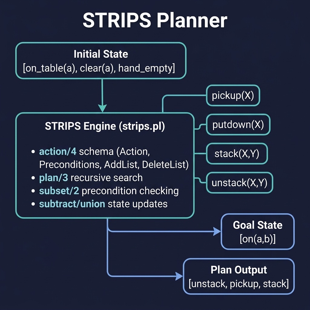
The strips_planner project implements the core algorithm and two practical variants. Here is the file strips_planner/prolog/strips.pl:
 1 %% strips.pl - STRIPS-style planner with multiple domains
 2 :- module(strips, [
 3     plan/3,
 4     plan_bfs/3,
 5     plan_visited/3
 6 ]).
 7
 8 %% holds(+Conditions, +State)
 9 %% True when every condition in Conditions is present in State.
10 %% Uses member/2 (not memberchk) so that variables in Conditions
11 %% can be bound to any matching element in State.
12 holds([], _).
13 holds([C|Cs], State) :- member(C, State), holds(Cs, State).
14
15 %% plan(+InitState, +GoalState, -Plan)
16 %% Depth-first search through the state space.
17 plan(State, Goal, []) :-
18     holds(Goal, State).
19 plan(State, Goal, [Action|Plan]) :-
20     action(Action, Preconditions, AddList, DeleteList),
21     holds(Preconditions, State),
22     subtract(State, DeleteList, TempState),
23     union(TempState, AddList, NewState),
24     plan(NewState, Goal, Plan).
25
26 %% plan_bfs(+InitState, +GoalState, -Plan)
27 %% Breadth-first search — guaranteed to find the shortest plan.
28 plan_bfs(State, Goal, Plan) :-
29     plan_bfs_queue([bfs_node(State, [])], Goal, RevPlan),
30     reverse(RevPlan, Plan).
31
32 plan_bfs_queue([bfs_node(State, Actions)|_], Goal, Actions) :-
33     holds(Goal, State), !.
34 plan_bfs_queue([bfs_node(State, Actions)|Rest], Goal, Plan) :-
35     findall(
36         bfs_node(NewState, [Action|Actions]),
37         (   action(Action, Preconditions, AddList, DeleteList),
38             holds(Preconditions, State),
39             subtract(State, DeleteList, TempState),
40             union(TempState, AddList, NewState)
41         ),
42         Children
43     ),
44     append(Rest, Children, NewQueue),
45     plan_bfs_queue(NewQueue, Goal, Plan).
46
47 %% plan_visited(+InitState, +GoalState, -Plan)
48 %% DFS with cycle detection — avoids revisiting states.
49 plan_visited(State, Goal, Plan) :-
50     retractall(plan_visited_state(_)),
51     plan_visited_dfs(State, Goal, [], Plan).
52
53 :- dynamic plan_visited_state/1.
54
55 plan_visited_dfs(State, Goal, _ActionPath, []) :-
56     holds(Goal, State), !.
57 plan_visited_dfs(State, Goal, ActionPath, [Action|Plan]) :-
58     action(Action, Preconditions, AddList, DeleteList),
59     holds(Preconditions, State),
60     subtract(State, DeleteList, TempState),
61     union(TempState, AddList, NewState),
62     \+ plan_visited_state(NewState),
63     assert(plan_visited_state(NewState)),
64     plan_visited_dfs(NewState, Goal, [Action|ActionPath], Plan).
How the Planner Works
The planner provides three search strategies, all built on the same action interface:
Depth-first search (plan/3) is the simplest: recursively try every applicable action, building the plan as Prolog backtracks. With only 10 lines of logic it captures the essence of STRIPS planning — but it may loop forever when actions are reversible (you can pick up a block and put it down indefinitely).
Breadth-first search (plan_bfs/3) maintains an explicit queue of bfs_node(State, RevActions) terms. It expands all nodes at depth d before any at depth d+1, guaranteeing the first plan found has the minimum number of actions. The trade-off is memory: the queue can grow large for complex problems.
DFS with cycle detection (plan_visited/3) stores visited states in a dynamic predicate and skips any state already encountered. This avoids the infinite-loop problem of naive DFS while retaining its space efficiency. It does not guarantee optimality, but in practice it finds reasonable plans quickly.
The holds/2 Predicate
A subtle but critical detail: we define holds/2 using member/2 rather than SWI-Prolog’s built-in subset/2. The built-in uses memberchk/2, which is semi-deterministic — it commits to the first matching element in the state. This means a variable like X in an action schema pickup(X) would always bind to the first block found, and findall would never discover actions for other blocks. By using member/2, we allow Prolog to backtrack and try every possible binding for action-schema variables.
Running the Planner
Here is a simple blocks-world query using the DFS planner:
1 ?- plan([on_table(a), clear(a), hand_empty], [holding(a)], Plan).
2 Plan = [pickup(a)].
For the two-block stacking problem, BFS finds the optimal 2-step plan:
1 ?- plan_bfs([on_table(a), on_table(b), clear(a), clear(b), hand_empty],
2             [on(a, b)], Plan).
3 Plan = [pickup(a), stack(a, b)].
Building a three-block tower, BFS finds the minimal 4-step sequence:
1 ?- plan_bfs([on_table(a), on_table(b), on_table(c),
2              clear(a), clear(b), clear(c), hand_empty],
3             [on(a, b), on(b, c)], Plan).
4 Plan = [pickup(b), stack(b, c), pickup(a), stack(a, b)].
Domain Definitions
The same planner works for any domain once the actions are defined. The blocks world uses four operators:
1 action(pickup(X),
2     [on_table(X), clear(X), hand_empty],
3     [holding(X)],
4     [on_table(X), clear(X), hand_empty]).
5
6 action(stack(X, Y),
7     [holding(X), clear(Y)],
8     [on(X, Y), clear(X), hand_empty],
9     [holding(X), clear(Y)]).
The logistics domain, with trucks and planes moving packages, uses distinct predicate names (pkg_at/2, truck_at/2, plane_at/2) so that action-schema variables bind to the correct entity types:
1 action(load_truck(Pkg, Truck, Loc),
2     [pkg_at(Pkg, Loc), truck_at(Truck, Loc), free(Truck)],
3     [in(Pkg, Truck)],
4     [pkg_at(Pkg, Loc), free(Truck)]).
5
6 action(drive(Truck, From, To),
7     [truck_at(Truck, From), road(From, To)],
8     [truck_at(Truck, To)],
9     [truck_at(Truck, From)]).
A logistics query — shipping a package from loc_a to loc_b using a truck:
1 ?- plan_bfs([pkg_at(pkg1, loc_a), truck_at(truck1, loc_a), free(truck1),
2              road(loc_a, loc_b), road(loc_b, loc_a)],
3             [pkg_at(pkg1, loc_b)], Plan).
4 Plan = [load_truck(pkg1, truck1, loc_a),
5         drive(truck1, loc_a, loc_b),
6         unload_truck(pkg1, truck1, loc_b)].
This separation of planner from domain is the key architectural insight: add a new domain by defining action/4 facts and the search code never changes.
The Blocks World
The blocks world is the classic AI planning domain: a robot arm manipulates labeled blocks on a table, stacking and unstacking them to achieve a goal configuration. The domain is simple enough to reason about formally yet rich enough to demonstrate core planning challenges: search, state representation, and the frame problem.
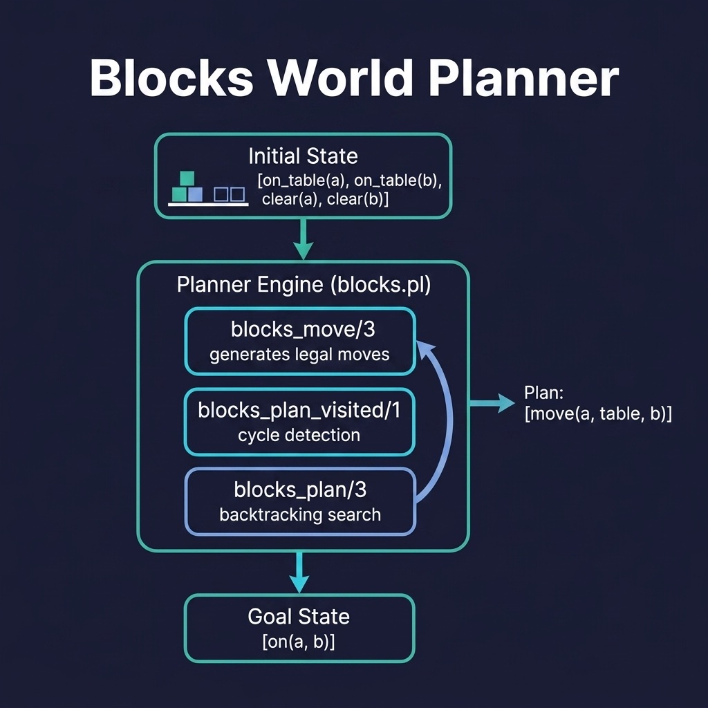
While the generic STRIPS planner above can solve blocks-world problems, the dedicated blocks_world project uses a more natural move representation and adds cycle detection. Here is the file blocks_world/prolog/blocks.pl:
 1 %% blocks.pl - Blocks World planner
 2 :- module(blocks, [
 3     blocks_plan/3,
 4     print_state/1
 5 ]).
 6
 7 %% blocks_plan(+InitState, +GoalState, -Moves)
 8 %% State is a list of on(X,Y) and on_table(X) atoms
 9 blocks_plan(State, Goal, []) :-
10     subset(Goal, State), !.
11 blocks_plan(State, Goal, [Move|Moves]) :-
12     blocks_move(State, Move, NewState),
13     \+ blocks_plan_visited(NewState),
14     assert(blocks_plan_visited(NewState)),
15     blocks_plan(NewState, Goal, Moves).
16
17 :- dynamic blocks_plan_visited/1.
18
19 blocks_move(State, move(X, table, To), NewState) :-
20     member(on_table(X), State),
21     clear(X, State),
22     block_in_state(To, State),
23     dif(X, To),
24     clear(To, State),
25     select(on_table(X), State, S1),
26     NewState = [on(X, To)|S1].
27 blocks_move(State, move(X, From, To), NewState) :-
28     member(on(X, From), State),
29     clear(X, State),
30     block_in_state(To, State),
31     dif(X, To),
32     clear(To, State),
33     select(on(X, From), State, S1),
34     NewState = [on(X, To)|S1].
35 blocks_move(State, move_to_table(X, From), NewState) :-
36     member(on(X, From), State),
37     clear(X, State),
38     select(on(X, From), State, S1),
39     NewState = [on_table(X)|S1].
40
41 block_in_state(B, State) :- member(on_table(B), State).
42 block_in_state(B, State) :- member(on(B, _), State).
43 block_in_state(B, State) :- member(on(_, B), State).
44
45 clear(X, State) :- \+ member(on(_, X), State).
46 clear(table, _).
Design Decisions
Several choices distinguish this dedicated planner from the generic STRIPS version:
Move representation. Rather than STRIPS-style add/delete lists, blocks_move/3 works directly with state lists. The select/3 predicate removes the block from its old position and the new on/2 or on_table/1 term is prepended to form the new state. This is more concise for this specific domain and produces human-readable move descriptions like move(a, table, b).
Cycle detection. The blocks_plan_visited/1 dynamic predicate records every visited state. Before exploring a move, the planner checks that the resulting state has not already been seen. This prevents the infinite loops that naive DFS would encounter — without it, the planner could move a block back and forth between the same two positions forever.
The clear/2 rule. A block is clear when nothing is stacked on top of it. The rule clear(X, State) :- \+ member(on(_, X), State) uses negation-as-failure: X is clear if there is no block Y such that on(Y, X) holds. The table is always clear.
State representation. States are simple lists of on(X, Y) and on_table(X) atoms. The goal is a list of atoms that must all be present in the final state — typically just the desired on/2 relationships, ignoring table facts.
Example Queries
Stack block a on top of block b starting from an empty table:
1 ?- blocks_plan([on_table(a), on_table(b), clear(a), clear(b)],
2                [on(a, b)], Moves).
3 Moves = [move(a, table, b)].
Rearrange a small tower by unstacking a from b and restack b on a:
1 ?- blocks_plan([on(a, b), on_table(b), clear(a)],
2                [on(b, a)], Moves).
3 Moves = [move(a, b, table), move(b, table, a)].
The dedicated representation produces plans that read naturally: “move block a from b to the table, then move block b from the table to a.”
Planning with Constraints
Classical STRIPS planning answers what to do, but real-world problems also demand answers to when and with what resources. Constraint Logic Programming over finite domains (CLP(FD)) extends planning with temporal reasoning, resource limits, and scheduling constraints, all while retaining Prolog’s declarative style.
Temporal Constraints on Actions
In a pure STRIPS plan, actions have no duration and execute instantaneously. Adding time transforms planning into scheduling: each action occupies a time interval, and these intervals must respect ordering and resource constraints.
The CLP(FD) approach models each action’s start time as a finite-domain variable:
- Precedence: If action B must follow action A, constrain
StartB #>= EndA. - Deadlines: If an action must finish by time T, constrain
End #=< T. - Duration:
End #= Start + Duration.
These integer constraints propagate through the constraint network. When a start time’s domain is reduced, the solver automatically tightens the domains of linked actions — pruning the search space before any concrete time is assigned.
Hybrid Planning and Scheduling
A practical architecture separates the two concerns:
- A STRIPS planner (like the ones in the previous sections) finds a valid action sequence.
- A constraint solver assigns times and resources to that sequence.
This division works because the causal structure (what actions are needed and in what order) is often independent of the temporal structure (exactly when each action executes). For problems where action choice depends on timing, such as selecting a faster but costlier machine over a slower cheaper one, the two layers can interleave: the planner proposes a partial plan, the scheduler checks feasibility, and backtracking drives the combined search.
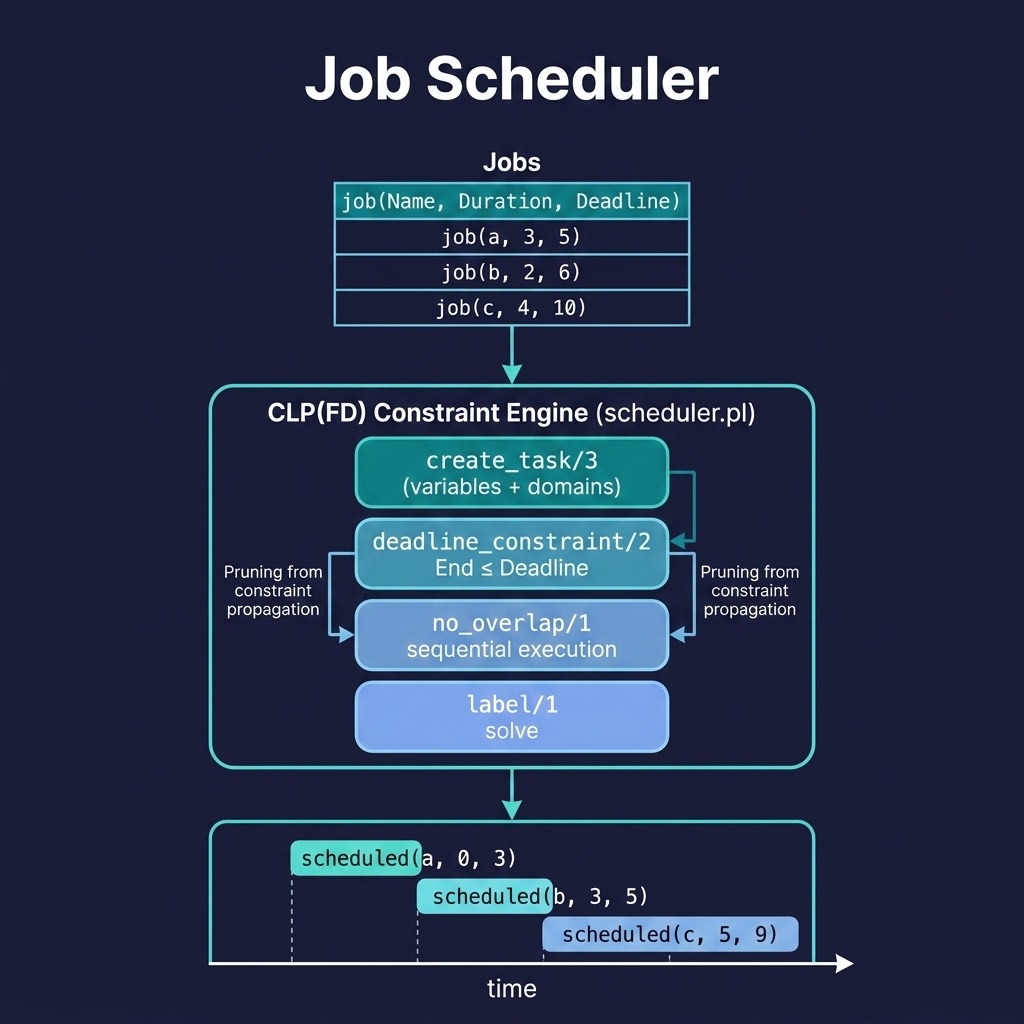
A Constraint-Based Scheduler
The companion project job_scheduler (described fully in the Constraint Logic Programming chapter) demonstrates the scheduling layer. Here is the file job_scheduler/prolog/scheduler.pl:
 1 schedule_jobs(Jobs, Schedule) :-
 2     maplist(create_task, Jobs, Schedule, Starts),
 3     chain(Starts, #=<),          % order tasks by start time
 4     maplist(deadline_constraint, Jobs, Schedule),
 5     no_overlap(Schedule),        % one job at a time
 6     maplist(label_task, Schedule).
 7
 8 create_task(job(Name, Duration, _Deadline), scheduled(Name, Start, End),
 9     Start) :-
10     Start in 0..100,
11     End #= Start + Duration.
12
13 no_overlap([]).
14 no_overlap([_]).
15 no_overlap([scheduled(_,_,End1)|Rest]) :-
16     Rest = [scheduled(_,Start2,_)|_],
17     End1 #=< Start2,
18     no_overlap(Rest).
This scheduler handles three constraint types simultaneously:
- Capacity:
no_overlap/1ensures only one job executes at a time on the shared machine. - Deadlines: each job’s
Endmust not exceed its deadline. - Ordering:
chain/2sorts jobs by start time, eliminating symmetries.
A six-job problem with tight deadlines:
1 ?- schedule_jobs([job(a, 3, 5), job(b, 2, 6), job(c, 4, 10),
2                   job(d, 1, 11), job(e, 2, 13), job(f, 5, 18)], Schedule).
3 Schedule = [scheduled(a,0,3), scheduled(b,3,5), scheduled(c,5,9),
4             scheduled(d,9,10), scheduled(e,10,12), scheduled(f,12,17)].
The constraint solver finds a feasible packing where short tasks d and e fill gaps between longer jobs: a pattern that appears in real production scheduling, timetabling, and project planning.
Partial-Order Planning
Total-order planners (like the STRIPS examples above) produce fully ordered sequences of actions. But many actions are independent: moving a package from Boston to Chicago and loading a different truck in Seattle can happen in either order, or simultaneously. Partial-order planning (POP) exploits this independence, producing a plan as a set of actions with ordering constraints only where necessary.
Causal Links and Threats
A partial-order plan is a directed acyclic graph where:
- Nodes are actions, plus two special nodes: Start (producing the initial state) and Finish (requiring the goal).
- Ordering constraints specify that action A must precede action B.
- Causal links record that action A produces fluent p for action B to consume. Written as A ⟶^p B, a causal link means “A achieves precondition p of B.”
Planning proceeds by selecting an open precondition, a fluent needed by some action that is not yet linked to a producer, and either:
- Find an existing action whose effects include that fluent and add a causal link, or
- Add a new action to the plan that produces it.
Adding a causal link can create a threat: an action C that deletes the linked fluent and could be ordered between A and B. Threats are resolved by promotion (ordering C before A) or demotion (ordering C after B). If neither is possible, the plan is abandoned and the planner backtracks.
Why Partial-Order Planning Matters
POP produces least-commitment plans. By not imposing unnecessary orderings, the resulting plan admits many valid linearizations. This matters when:
- Multiple agents execute the plan concurrently — independent actions can truly run in parallel.
- Uncertain durations mean a later action might become ready before an earlier one completes.
- Replanning is needed mid-execution — an unordered action pair can be swapped without invalidating the plan.
Implementing POP in Prolog
Prolog’s unification and backtracking map cleanly onto the POP algorithm. A partial plan can be represented as a structure:
1 plan(Actions, Orderings, CausalLinks, OpenPreconditions)
The main loop selects an open precondition, nondeterministically chooses a resolver, adds the necessary ordering and causal-link constraints, checks for and resolves threats, and recurses. Prolog’s backtracking handles the nondeterministic choice of resolver — when threat resolution fails, the system automatically tries the next option.
While a full POP implementation is beyond the scope of this chapter, the key data structures sketch the approach:
 1 %% A causal link: Producer achieves Precondition for Consumer
 2 causal_link(Producer, Precondition, Consumer)
 3
 4 %% A threat: Deleter deletes Precondition, which is protected
 5 %% by a causal link from Producer to Consumer
 6 threat(Deleter, Precondition, Producer, Consumer)
 7
 8 %% Resolve a threat by ordering Deleter before Producer (promotion)
 9 %% or after Consumer (demotion), if consistent with existing orderings
10 resolve_threat(Threat, Plan, NewPlan) :-
11     (   promote(Threat, Plan, NewPlan)
12     ;   demote(Threat, Plan, NewPlan)
13     ).
The central insight is that partial-order planning generates a family of linear plans in a single search — every topological sort of the final plan graph is a valid execution. This compact representation is one of POP’s main advantages over total-order search.
Practical Job Scheduling Applications
Planning and scheduling techniques extend well beyond toy blocks and packages. This section surveys real-world applications where Prolog’s combined planning and constraint-solving capabilities offer significant leverage.
Project Scheduling with Resource Constraints
Construction projects, software releases, and manufacturing pipelines all share a common structure: tasks with durations, precedence requirements, and limited shared resources (crews, machines, specialists). The constraint-based approach from earlier sections scales to these problems:
- Resource pools replace the single-machine assumption. Instead of
no_overlap/1constraining all tasks, a cumulative constraint ensures that the sum of resource demands at any time does not exceed capacity:cumulative(Tasks, ResourceDemands, Capacity). - Precedence networks capture task dependencies: “the foundation must be poured before the framing begins.” These are modeled as
StartB #>= EndAconstraints, just like in the job scheduler. - Milestone deadlines anchor the schedule to calendar dates: the product launch, the conference deadline, the regulatory filing date.
Timetabling
University course scheduling, conference programs, and employee shift assignment are all instances of timetabling — assigning events to time slots and rooms while respecting hard constraints (no room double-booking, instructor availability) and soft preferences (consecutive lectures in the same building).
Prolog approaches timetabling by generating candidate assignments and using CLP(FD) to check feasibility. The constraint model captures rules like “Professor Smith cannot teach before 10 AM” (domain restriction on start-time variables) and “Room 101 seats 50, so classes with more than 50 students cannot be assigned there” (reification: if enrollment > 50 then room ≠ 101).
Integration with External Solvers
For industrial-scale scheduling, Prolog often serves as the modeling and orchestration layer rather than the raw solver. The Prolog program:
- Reads the problem specification (tasks, resources, constraints) from a database or file.
- Builds a constraint model in Prolog using CLP(FD) for rapid prototyping.
- For production, exports the model to a dedicated solver (OR-Tools, CPLEX, Gurobi) via a file interface or foreign function binding.
- Reads back the solution and validates it against the original constraints.
This architecture combines Prolog’s strengths — readable constraint formulation, rapid iteration, built-in search — with the raw speed of C++ solvers for large problem instances. The SWI-Prolog ecosystem supports this pattern through its C foreign interface and libraries for common data exchange formats.
The Prolog Advantage
Why use Prolog for scheduling at all? Three reasons stand out:
- Declarative constraints read like the problem description. “Task A ends before Task B starts” becomes
EndA #=< StartB— no manual implementation of search or propagation. - Backtracking is built in. When a partial schedule proves infeasible, Prolog automatically unwinds to the last choice point and tries an alternative — no hand-coded backtracking stack.
- Rapid prototyping. A working scheduler can be built in under 50 lines of Prolog. While a C++/CPLEX solution may run faster on 10,000 tasks, the Prolog version is running and validated long before the C++ version compiles.
Optional Practice Problems
- STRIPS Negative Preconditions: In the
strips_plannerproject, modify the planner to support negative preconditions (e.g., an action can only be performed if a state property is not true). - Resource Conflicts: In
job_scheduler, add a constraint limiting the number of available workers. Modify the scheduler to resolve overlapping jobs by delaying jobs when the worker limit is exceeded.