Constraint Logic Programming
Constraint Logic Programming (CLP) extends Prolog with the ability to reason about constraints over various domains — integers, reals, and finite domains. SWI-Prolog provides excellent CLP libraries that make it possible to solve complex combinatorial and optimization problems declaratively.
Introduction to CLP
In traditional logic programming, evaluation relies on unification and backtracking. For complex search problems, this often leads to a generate-and-test strategy: the program instantiates variables to concrete values and then checks if they satisfy the problem conditions. If they do not, it backtracks and tries other values. For large combinatorial search spaces, this approach is extremely inefficient.
Constraint Logic Programming (CLP) replaces this with a constrain-and-generate paradigm:
- Constraints are declarative relations that restrict the set of possible values (domains) that variables can take.
- The Constraint Solver maintains these relations. As soon as a variable’s domain is reduced, the solver automatically propagates this restriction to other related variables, narrowing their domains before concrete values are ever assigned. This process is called constraint propagation.
- By pruning branches of the search tree early, CLP turns NP-complete search problems into highly efficient deterministic operations, separating the description of the constraints from the search logic.
CLP(FD): Constraints over Finite Domains
Finite Domain constraint solving, or CLP(FD), deals with variables whose values are restricted to discrete, finite sets of integers. In SWI-Prolog, this is implemented in library(clpfd).
Unlike ordinary arithmetic operators (like is/2 or =:=/2), which require all variables to be fully bound to values, CLP(FD) relations are bidirectional and can evaluate partially instantiated variables.
Core CLP(FD) Predicates
in/2andins/2: Define the domain for a single variable or a list of variables (e.g.,X in 1..9,Vars ins 1..9).#=: Constraint equality.#\=: Constraint inequality.#<,#>,#=<,#>=: Constraint arithmetic comparisons.all_distinct(+List): A high-performance constraint asserting that all integers in the list must be unique.label(+List): Triggers backtracking search to instantiate variables to concrete values from their remaining domains.transpose(+Matrix, -Transposed): Transposes a 2D list matrix, crucial for grid-based constraints (such as column checks).
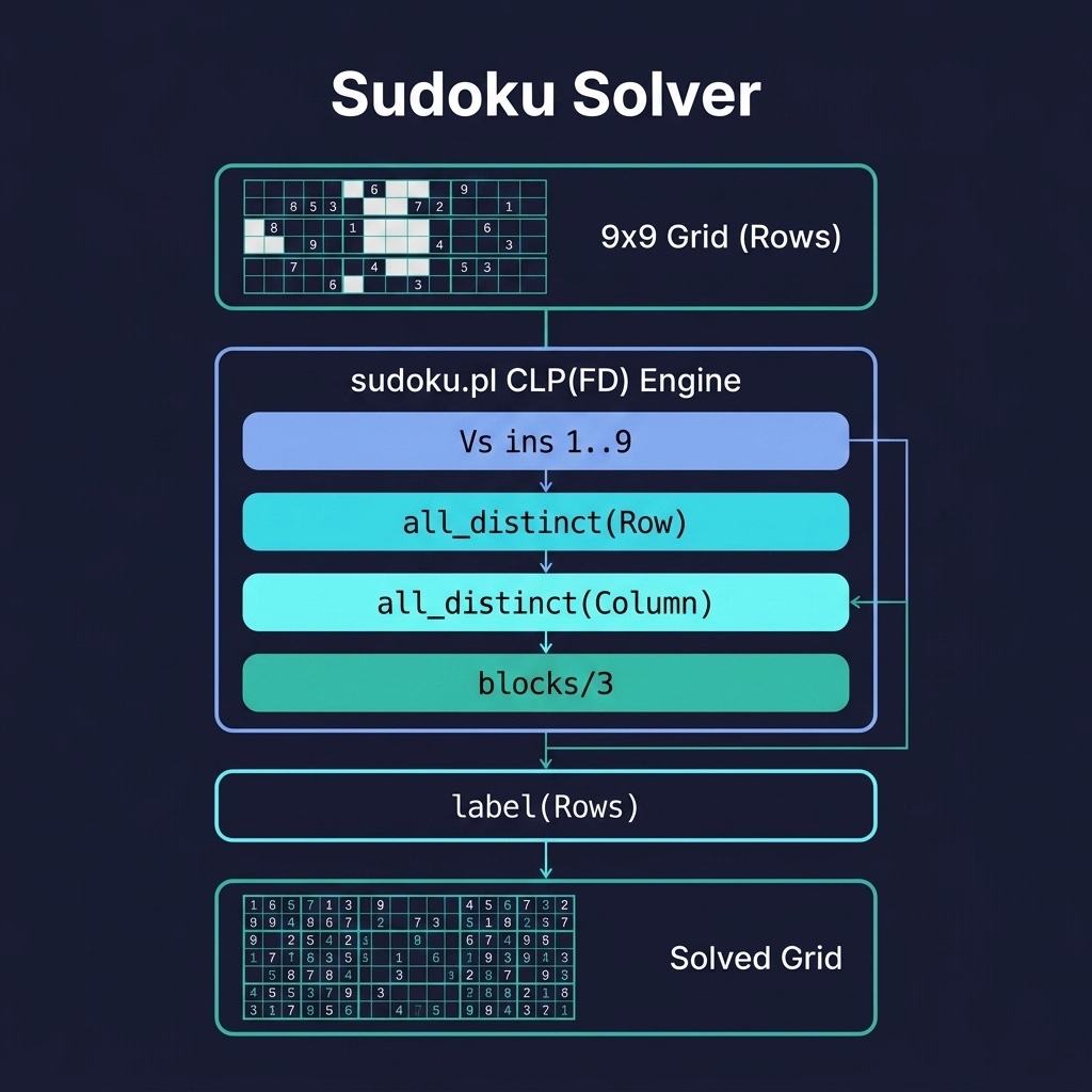
Solving Sudoku with CLP(FD)
A classic demonstration of constraint propagation is solving Sudoku puzzles. Standard Sudoku requires placing digits 1 to 9 in a  grid such that every row, column, and
  sub-grid block contains unique numbers.
Using library(clpfd), we can model this complete constraint system in under 20 lines of logic. The solver propagates constraints so efficiently that most puzzles are solved instantly without any backtracking search at all.
The sudoku_solver project provides a complete solver in under 30 lines of logic. Here is the file sudoku_solver/prolog/sudoku.pl:
 1 :- module(sudoku, [
 2     sudoku/1,
 3     print_board/1
 4 ]).
 5
 6 :- use_module(library(clpfd)).
 7
 8 %% sudoku(+Rows) - Solve a 9x9 Sudoku puzzle
 9 %% Rows is a list of 9 lists, each containing 9 elements (vars or 1-9)
10 sudoku(Rows) :-
11     length(Rows, 9),
12     maplist(same_length(Rows), Rows),
13     append(Rows, Vs), Vs ins 1..9,
14     maplist(all_distinct, Rows),
15     transpose(Rows, Columns),
16     maplist(all_distinct, Columns),
17     Rows = [As,Bs,Cs,Ds,Es,Fs,Gs,Hs,Is],
18     blocks(As, Bs, Cs),
19     blocks(Ds, Es, Fs),
20     blocks(Gs, Hs, Is),
21     maplist(label, Rows).
22
23 blocks([], [], []).
24 blocks([N1,N2,N3|Ns1], [N4,N5,N6|Ns2], [N7,N8,N9|Ns3]) :-
25     all_distinct([N1,N2,N3,N4,N5,N6,N7,N8,N9]),
26     blocks(Ns1, Ns2, Ns3).
27
28 %% print_board(+Rows) - Pretty-print a solved board
29 print_board([]).
30 print_board([Row|Rows]) :-
31     format("~w~n", [Row]),
32     print_board(Rows).
The N-Queens Problem
The N-Queens problem asks how to place  non-attacking queens on an
  chessboard.
- Naive Backtracking: Places a queen row-by-row, recursively checking for row, column, and diagonal conflicts. If a conflict is found, it backtracks. This checks many invalid states.
- CLP(FD) Search: Declares queen positions as variables, constrains their columns and diagonals, and uses constraint propagation to prune invalid domains before values are labeled. This limits backtracking.
The diagonal constraints are written using arithmetic offsets: two queens at columns  and
and  separated by
  rows are on the same diagonal if
  , which translates to
 Q #\= Q1 + D and Q #\= Q1 - D.
The n_queens project solves the problem using CLP(FD) diagonal constraints. Here is the file n_queens/prolog/queens.pl:
 1 %% queens.pl - N-Queens solver using CLP(FD)
 2 :- module(queens, [
 3     n_queens/2
 4 ]).
 5
 6 :- use_module(library(clpfd)).
 7
 8 %% n_queens(+N, -Queens)
 9 %% Queens is a list of column positions for queens in each row
10 n_queens(N, Queens) :-
11     length(Queens, N),
12     Queens ins 1..N,
13     safe_queens(Queens),
14     label(Queens).
15
16 safe_queens([]).
17 safe_queens([Q|Qs]) :-
18     safe_queen(Q, Qs, 1),
19     safe_queens(Qs).
20
21 safe_queen(_, [], _).
22 safe_queen(Q, [Q1|Qs], D) :-
23     Q #\= Q1,
24     Q #\= Q1 + D,
25     Q #\= Q1 - D,
26     D1 #= D + 1,
27     safe_queen(Q, Qs, D1).
Scheduling and Resource Allocation
Scheduling tasks with deadlines, resource limitations, and ordering constraints is a classic industrial optimization problem.
- Precedence constraints: Task B must start after Task A ends (
StartB #>= EndA). - Resource constraints: Two tasks using the same resource cannot overlap in time.
- Deadline constraints: Tasks must complete before a specific time limit.
CLP(FD) lets you express these temporal equations naturally, solving complex scheduling problems by treating start and end times as integer variables.
The job_scheduler project models scheduling with temporal constraints. Here is the file job_scheduler/prolog/scheduler.pl:
 1 %% scheduler.pl - Job scheduling with temporal constraints using CLP(FD)
 2 :- module(scheduler, [
 3     schedule_jobs/2,
 4     no_overlap/1
 5 ]).
 6
 7 :- use_module(library(clpfd)).
 8
 9 %% schedule_jobs(+Jobs, -Schedule)
10 %% Jobs: list of job(Name, Duration, Deadline) terms
11 %% Schedule: list of scheduled(Name, Start, End) terms
12 schedule_jobs(Jobs, Schedule) :-
13     maplist(create_task, Jobs, Schedule, Starts),
14     chain(Starts, #=<),  % order tasks by start time
15     maplist(deadline_constraint, Jobs, Schedule),
16     no_overlap(Schedule),
17     maplist(label_task, Schedule).
18
19 create_task(job(Name, Duration, _Deadline), scheduled(Name, Start, End),
20     Start) :-
21     Start in 0..100,
22     End #= Start + Duration.
23
24 deadline_constraint(job(Name, _Duration, Deadline), scheduled(Name,
25     _Start, End)) :-
26     End #=< Deadline.
27
28 no_overlap([]).
29 no_overlap([_]).
30 no_overlap([scheduled(_,_,End1)|Rest]) :-
31     Rest = [scheduled(_,Start2,_)|_],
32     End1 #=< Start2,
33     no_overlap(Rest).
34
35 label_task(scheduled(_, Start, _)) :- label([Start]).
CLP(R) and CLP(Q): Constraints over Reals and Rationals
While CLP(FD) is designed for discrete integers, SWI-Prolog also provides constraint solvers over continuous domains:
library(clpr): Constraints over Real numbers.library(clpq): Constraints over Rational numbers.
These libraries use the Simplex algorithm under the hood to solve systems of linear equations and inequalities, propagating constraints across real-valued variables.
Example: Simultaneous Equations
We can express continuous equations using curly brace { ... } syntax:
1 ?- use_module(library(clpr)).
2
3 ?- {X + Y =:= 10, X - Y =:= 4}.
4 X = 7.0,
5 Y = 3.0.
CLP(R) is widely used in engineering (e.g., electrical circuit analysis), financial modeling, and optimization where variables represent continuous values like currency, voltage, or distance.
CLP(B): Boolean Constraints
Boolean constraint solving, or CLP(B), operates on boolean variables (restricted to the values 0 for false and 1 for true). It is implemented in library(clpb).
CLP(B) uses Binary Decision Diagrams (BDDs) to represent and solve boolean formulas efficiently, making it powerful for Boolean Satisfiability (SAT) solving, combinatorial verification, and digital circuit design.
Example: Logic Gate Satisfiability
We can express logical operations (such as AND *, OR +, NOT ~, XOR #) and verify conditions:
1 ?- use_module(library(clpb)).
2
3 % Find values for X and Y that satisfy (X AND Y = 1)
4 ?- sat(X * Y =:= 1).
5 X = 1,
6 Y = 1.
Optional Practice Problems
- Cryptarithmetic Solver: In the
sudoku_solverorn_queensproject directories, create a new file that solves the classic cryptarithmetic puzzleSEND + MORE = MONEYusing CLP(FD) constraints. - Variable Board Size: Modify the N-Queens solver in
n_queensto run dynamically for any board sizeNsupplied at the query prompt, profiling the performance differences between smaller and larger boards.