Probabilistic Logic Programming

Probabilistic logic programming combines the expressiveness of Prolog with the ability to reason under uncertainty. SWI-Prolog supports several probabilistic programming frameworks that are highly relevant for modern AI applications. We look at a simple example in this chapter and then take a more general look at probability in the next chapter.

In classical logic, a statement is either true or false. This binary worldview works well for pure mathematics but fails in real-world AI applications where information is almost always incomplete, noisy, or uncertain.

Classical Prolog relies on the Closed World Assumption: if a fact cannot be proven true from the knowledge base, it is assumed to be false. However, in the real world, a lack of evidence does not equal evidence of absence. Furthermore, classical logic is monotonic: once a fact is proven, it remains true regardless of any new information added to the system.

In contrast, real-world reasoning is non-monotonic and probabilistic. For instance, we might believe a patient has a specific illness with certainty, but when a new test result comes back negative, our belief should adapt. Probabilistic logic programming solves this by representing truth values as real numbers in the range , representing the probability or degree of belief that a statement holds. This allows us to build logic models that handle exceptions, noisy measurements, and uncertain outcomes.

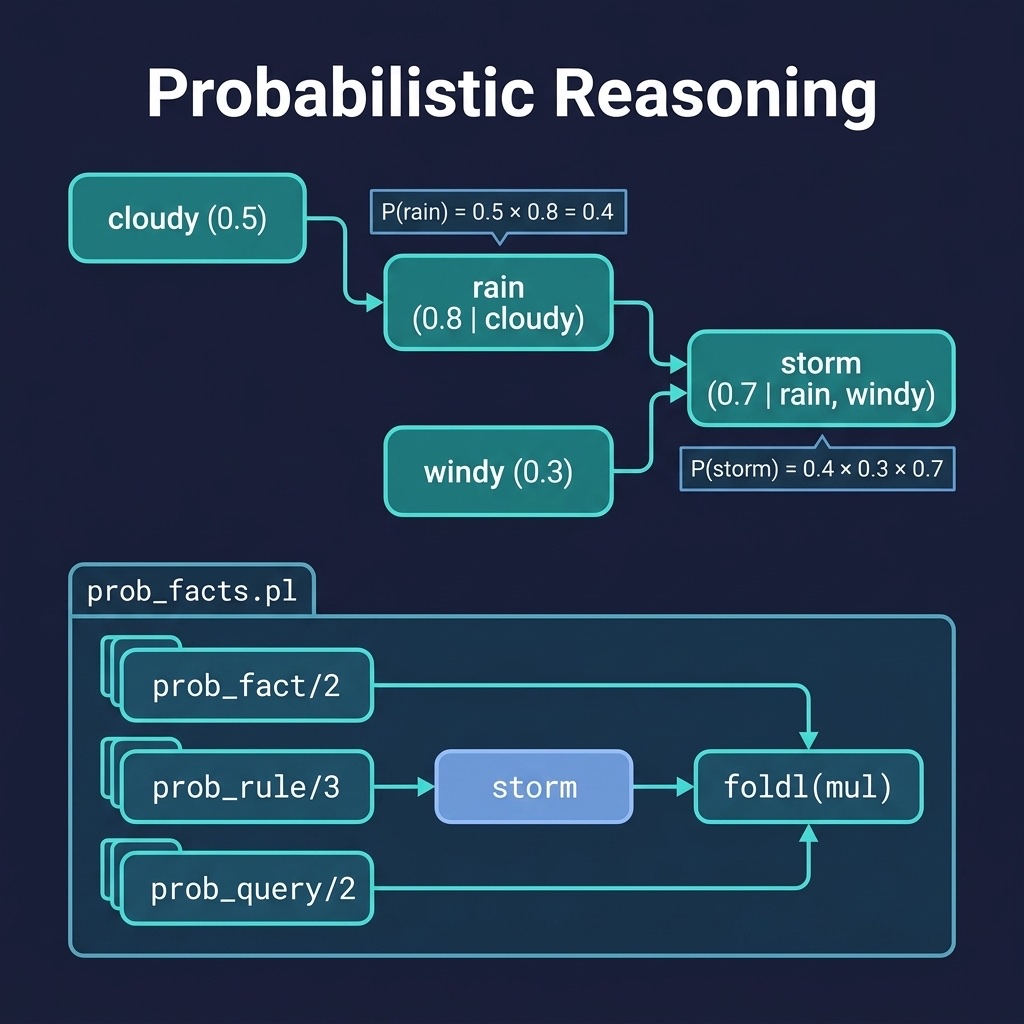
One of the most popular frameworks for combining logic with probability is ProbLog. In ProbLog, facts can be annotated with their probability of being true:

This notation declares that windy has a chance of being true, and cloudy has a chance. Under the distribution semantics introduced by Taisuke Sato, a ProbLog program defines a probability distribution over a set of possible worlds. In each possible world, every probabilistic fact is independently chosen to be either true (with probability ) or false (with probability ). The probability of a query is the sum of the probabilities of all possible worlds in which the query can be logically proven.

While a full ProbLog solver requires compiling queries into Binary Decision Diagrams (BDDs) to handle dependencies and logical cycles, we can implement a lightweight reasoner using certainty factors in pure Prolog. This approach propagates probabilities recursively through backtracking search.

The prob_reasoning project implements a lightweight probabilistic reasoner. Here is the file prob_reasoning/prolog/prob_facts.pl:

• Facts and Rules: The reasoner defines probabilistic facts using prob_fact(Fact, Probability) and conditional rules using prob_rule(Conditions, Goal, CondProb).
• Query Propagation: The prob_query/2 predicate calculates the probability of a goal:
  1. If the goal matches a base fact directly, it returns that probability.
  2. If the goal is derived via a rule, it recursively calls prob_query/2 on all conditions in the rule’s body using maplist/3.
  3. It then multiplies all the condition probabilities together using foldl/4 and the mul/3 helper to compute the JointProb of the preconditions.
  4. Finally, the joint probability is multiplied by the rule’s conditional probability (CondProb) to get the final goal probability.

The weather knowledge base demonstrates how probabilities attenuate (rapidly decrease) across deep inference chains. Consider the path from low_pressure to tornado_risk:

1. low_pressure is a base fact with .
2. unstable_air is derived from low_pressure with conditional probability , yielding .
3. thick_clouds is derived from high_humidity () and unstable_air () with conditional probability , yielding .
4. Parallel reasoning yields frontal_zone () and storm_system ().
5. severe_storm converges from thick_clouds and storm_system with conditional probability , yielding .
6. tornado_risk is derived from severe_storm with conditional probability , yielding .

This rapid attenuation shows that naive multiplication across deep chains can quickly shrink probabilities. In real-world applications, to prevent underflow and model complex dependencies correctly, we use more sophisticated models like Bayesian networks or full ProbLog.

Writing down exact probability values for every fact and rule is difficult. In practice, we often have the logical structure of the model but need to learn the probability values from experimental data or observations.

This process is called parameter learning (implemented in ProbLog as LFI, or Learning from Interpretations). The learning system is given:

1. A logic program containing facts and rules with unknown probability parameters.
2. A database of training interpretations (examples of observed states, which may be complete or incomplete).

Under the hood, the system uses the Expectation-Maximization (EM) algorithm:

• Expectation Step (E-step): Using the current probability estimates, the system computes the expected truth values of all unobserved (latent) variables in the training data.
• Maximization Step (M-step): The system updates the probability parameters to maximize the likelihood of both the observed and expected data.

This iterative process continues until the parameters converge, allowing us to train probabilistic logic systems directly from tabular data, sensor logs, or historical records.

A Bayesian Network is a directed acyclic graph (DAG) where nodes represent random variables and edges represent conditional dependencies. Each node is associated with a Conditional Probability Table (CPT) expressing the probability of the node given the states of its parent nodes.

Prolog is well-suited for representing Bayesian networks. We can represent the network structure and CPTs directly as facts:

To perform inference (such as calculating ), we can write a query solver that uses variable elimination or enumeration to sum out the latent variables over the joint distribution:

P(A \mid B) = \frac{P(A, B)}{P(B)} = \frac{\sum_{Y} P(A, B, Y)}{\sum_{X, Y} P(X, B, Y)}

Prolog’s pattern matching and list processing make it easy to traverse parent-child relationships and lookup CPT probabilities during joint probability factorization.

Probabilistic logic programming has several unique strengths for real-world AI systems:

1. Fault Diagnosis under Uncertainty: Industrial systems contain many interconnected components. When a sensor reports a failure, we must diagnose the root cause. Since sensors are noisy and can fail themselves, probabilistic logic allows us to model rules like “If component X fails, sensor Y shows error with 95% probability, but sensor Y has a 2% random failure rate.” The inference engine can then identify the most likely failed component.

2. Medical Reasoning: Diseases and symptoms do not have a simple one-to-one mapping. A symptom can be caused by multiple diseases, and a disease does not always produce all symptoms. By modeling symptoms as probabilistic facts and diseases as conditional hypotheses, we can calculate the posterior probability of each diagnosis given a patient’s clinical file.

3. Information Extraction Pipelines: Modern NLP systems (like NER taggers or relation extractors) output extracted facts with confidence scores. By feeding these confidence scores directly into a probabilistic Prolog reasoner as probabilistic facts (e.g., 0.85::extracted_relation('ACME', 'acquired', 'BetaCorp')), we can run logical reasoning while correctly propagating the extraction uncertainty downstream to final conclusions.