Genetic Programming
Genetic programming (GP) is evolutionary search over programs. Ordinary machine learning fits numbers inside a model whose shape you choose. Genetic algorithms evolve fixed-length parameter vectors. GP goes one level up: it evolves the structure itself. The individual is a tree-shaped program, the training signal is a set of fitness cases (input/output examples of the behavior you want), and the operators of evolution build new programs out of parts of old ones.
John Koza established the field in the early 1990s with the observation that, given a function set, a terminal set, and a behavioral score, evolution discovers not only the coefficients of a formula but the formula. Three decades of later work refined the machinery (typed trees, linear representation, grammar-guided GP, geometric semantic crossover), but the core loop is small enough to implement in a few hundred lines of Python, which is exactly what you will do in this chapter.
We build everything from first principles, with no NumPy and no GP framework, and apply the same engine to four different problems:
| Example | Evolved object | Fitness cases |
|---|---|---|
| 1. Symbolic regression | math expression | 40 noisy (x, y) samples |
| 2. Boolean logic synthesis | gate netlist | 32-row truth table |
| 3. Regex synthesis | pattern program | 8 positive + 11 negative strings |
| 4. L-system plant | growth rule | cell grid of a target plant |
Run time for each demo is under three seconds on a laptop, and every run is seeded and reproducible.
This chapter assumes no prior exposure to genetic programming. We start with the ideas and the words, then build the engine, then run four complete problems with it. If you already know the field, skip ahead to “A tiny engine: gp_core.py”; everything before that section is background.
Where GP fits
Machine learning usually answers two questions in order:
- What shape should the model have? A line, a polynomial, a decision tree, a neural network.
- What numbers should that shape use? Coefficients, weights, thresholds.
Ordinary fitting answers only the second question. You choose the shape by hand, then a solver finds the numbers. It works spectacularly well when you already know the shape.
Genetic programming attacks the first question. The model is the program, and evolution finds both its structure and whatever constants it contains. Nothing is differentiated. The training signal is a score you compute by running each candidate on examples, so any behavior you can simulate can be optimized, whether or not it is smooth or continuous.
That matters most when the shape is the hard part:
- You have data and no idea what function produced it.
- You can simulate what you want to build, but you cannot write a differentiable loss for it.
- The answer has to be readable by a person, not a matrix of weights.
- The output is naturally discrete: a rule, a circuit, a regular expression, a schedule, a controller.
The price is that GP is a search, and the space it searches is astronomically large. Consider the simplest possible setup: four binary operators and two terminals. A perfect binary tree four levels deep has seven internal nodes and eight leaves, so there are 4^7 * 2^8, about 4.2 million, distinct programs of exactly that shape. At six levels the same count passes 10^28. GP also has to consider every irregular shape up to its depth limit, and there is no list to iterate through: it samples, scores, and breeds.
The three ingredients
Every evolutionary algorithm, GP included, needs three things:
- Variation. Something must create new candidates (random initialization, crossover, mutation).
- Heredity. Offspring must resemble their parents, or progress cannot accumulate (a tree is copied, then edited).
- Selection. Something must favor better candidates, or the population wanders (fitness, tournaments, elitism).
Remove any one of the three and the loop stops being evolution. Random search has variation but no heredity. Hill climbing has selection and heredity but almost no variation. GP has all three, applied to programs.
How GP differs from its neighbors
| Method | What is optimized | Uses gradients | Typical output |
|---|---|---|---|
| Least squares / logistic regression | coefficients | yes | numbers |
| Neural network training | weights | yes (backpropagation) | numbers |
| Genetic algorithm | a fixed-length vector | no | numbers |
| Genetic programming | program structure | no | a readable program |
| Bayesian optimization | a few continuous settings | no | numbers |
| Random or grid search | whatever you define | no | a sampled configuration |
| Large language model | text, from pretraining | no (pretraining only) | code or prose |
The last row deserves a sentence, because readers today will ask. A language model can propose a program from a description, but it has no loop that measures that program against your objective and improves it. GP has exactly that loop and no idea what your problem means. The two compose well: use a model to suggest a function set or seed the population, and let GP optimize against measurements. We return to that in “What GP is good at, and when not to reach for it”.
The vocabulary of evolution
GP borrows its words from biology. The mapping is loose but useful, and every GP paper and library uses these terms.
| Word | Meaning in GP | In this chapter |
|---|---|---|
| individual, program | one candidate solution | one Tree
|
| population | the individuals alive at one time | a list[Tree]
|
| generation | one round of selection and reproduction | one pass of the evolve() loop |
| genotype | the representation that is copied and varied | the tree itself |
| phenotype | the behavior the genotype produces | the formula, circuit, regex, or plant |
| gene, node | one part of the genotype | one Tree node |
| fitness | a number saying how well an individual solves the problem | the float that evolve() minimizes |
| fitness function | the procedure that computes fitness | the callable passed to evolve()
|
| fitness case | one test input, with its expected output | a data point, truth-table row, or example string |
| selection | choosing which individuals reproduce | tournament() |
| parent, offspring | who is copied, and the new individuals made from them | arguments and return values of crossover()
|
| crossover, recombination | mixing parts of two parents | crossover() |
| mutation | a random change to one individual |
mutate_subtree, mutate_point, mutate_hoist
|
| elitism | copying the best individuals forward unchanged | the elitism= argument |
| diversity | how different the individuals are | not measured here; it is what selection pressure trades away |
| convergence | the population becoming similar | visible as a flat history
|
| premature convergence | settling on a mediocre answer | example 1’s 37 stagnant generations |
| bloat | programs growing without getting better | fought with PARSIMONY, depth caps, and hoist mutation |
The one distinction to internalize is genotype versus phenotype. In example 4 the genotype is a rule tree of a few dozen nodes and the phenotype is a plant drawn on a 61 by 31 grid. Two different genotypes can produce the same phenotype, and the evolved rule and the hidden rule in that chapter draw exactly the same plant. Selection only ever sees the phenotype.
A note on signs: here “fitness” is a score we minimize, so lower is better. Many papers and libraries maximize it, so always check the convention before comparing numbers.
The shortest history of evolving programs
None of this is new. People have been trying to make computers evolve code since the 1950s.
Before the name
- In the 1950s, Nils Aall Barricelli ran some of the first computer simulations of evolution, letting numbers reproduce and compete on early machines.
- In 1957, A. S. Fraser simulated genetic systems on a digital computer, and in 1958 Richard Friedberg tried to evolve small programs by random mutation and selection. Both were ahead of their time and were largely forgotten for decades.
- In 1962, Hans-Joachim Bremermann wrote about optimization through evolution and recombination, the idea that a population of candidate solutions can search better than a single point.
- Through the 1960s a parallel thread appeared in Germany: evolution strategies, from Ingo Rechenberg and Hans-Paul Schwefel, tuned real-valued engineering parameters by mutation and selection.
Three classical branches
By the 1970s evolutionary computation had three schools that developed largely independently:
- Genetic algorithms, from John Holland’s 1975 book Adaptation in Natural and Artificial Systems. Binary, fixed-length strings; crossover was the star; the theory was built around schemata and building blocks. GP grew out of this branch.
- Evolution strategies, from Rechenberg and Schwefel: real vectors, self-adapting mutation step sizes, strong selection.
- Evolutionary programming, from Lawrence Fogel, Alvin Owens and Michael Walsh (1966): finite-state machines evolved by mutation, with no crossover at first.
The three differed in representation, in which operator they treated as primary, and in how much theory they carried, but they were running the same loop. Today “evolutionary computation” is the umbrella term for all of it, and researchers borrow freely across the branches.
From programs to genetic programming
In 1985, N. Michael Cramer published a representation for evolving simple sequential programs as trees, which is recognizably modern GP. The idea did not spread widely at the time.
In 1992, John Koza published Genetic Programming: On the Programming of Computers by Means of Natural Selection, and the field took off. Koza’s contribution was not one algorithm but a whole program of work:
- a clear tree representation with full, grow, and ramped half-and-half initialization;
- the operator mix of subtree crossover and mutation that the field still uses;
- a catalogue of benchmark problems, from symbolic regression (recovering the quartic polynomial
x^4 + x^3 + x^2 + x) and Boolean multiplexers to the “artificial ant” that follows the Santa Fe trail; - and, in later books (Genetic Programming II in 1994, III in 1999, and IV in 2003), the argument that GP routinely produces human-competitive results, including designs that won patents.
The infrastructure followed. The first European Workshop on Genetic Programming (EuroGP) was held in Paris in 1998, and GECCO, the main evolutionary computation conference, dates from the same period. Textbooks by Banzhaf, Nordin, Keller and Francone (1998) and Langdon and Poli (2002) turned the subject into a curriculum, and the free Field Guide to Genetic Programming (Poli, Langdon and McPhee, 2008) became the standard short introduction.
Where the field is now
Three decades of work added representations (linear programs, grammars, graphs, stacks), theory (why bloat happens, when GP can be expected to converge), and engineering (strongly typed nodes, semantic operators, multi-objective selection, GPU evaluation). Symbolic regression, GP’s oldest application, had a public moment in 2009, when Michael Schmidt and Hod Lipson used it to rediscover physical laws from measurements. Today the standard tools are libraries such as DEAP and gplearn, and a growing line of work uses large language models to propose programs or seed populations for GP to optimize. The loop itself has not changed.
| Year | Milestone |
|---|---|
| 1950s | Early evolutionary simulations (Barricelli) |
| 1957-1958 | First attempts to evolve programs (Fraser, Friedberg) |
| 1962 | Evolution and recombination as optimization (Bremermann) |
| 1960s | Evolution strategies (Rechenberg, Schwefel) and evolutionary programming (Fogel, Owens, Walsh) |
| 1975 | Genetic algorithms (Holland) |
| 1985 | Tree-shaped programs evolved (Cramer) |
| 1992 | Genetic programming named and popularized (Koza) |
| 1994 | Genetic Programming II (reusable subroutines); linear GP |
| 1998 | First EuroGP; grammatical evolution |
| 1999-2003 | Genetic Programming III and IV; human-competitive results |
| 2000s | Bloat theory; Cartesian, Push, and gene expression GP |
| 2009 | Symbolic regression rediscovers physical laws (Schmidt and Lipson) |
| 2010s | Semantic GP, multi-objective GP, mature Python libraries |
| 2020s | GP combined with machine learning and language models |
Why trees?
A GP individual is an ordered rooted tree. Internal nodes are functions (with a fixed arity), leaves are terminals (variables and constants). This single choice of representation drives almost everything else in the field, so it is worth understanding in detail.
A tree is a program
We write trees in prefix notation: a function name followed by its arguments. The tree
1             add
2           /     \
3         mul      sin
4        /   \       \
5       x    2.0      x
is written (add (mul x 2.0) (sin x)), which means x * 2.0 + sin(x). Prefix form removes two endless sources of bugs: there are no precedence rules to remember, and no parentheses to balance when you splice subtrees. The arity of each function decides the shape, so a well-formed tree is unambiguous by construction, and a subtree is always a complete expression on its own.
Two numbers describe a tree’s size. Size is the number of nodes; the tree above has size 7. Depth (also called height) is the longest root-to-leaf path counted in nodes; the tree above has depth 3, from add down to mul and then x. Every practical GP run limits at least one of these, or programs grow without bound.
The properties that make trees work
- Every subtree is a program. You can cut a subtree from one tree and graft it into another at any node, and the offspring is guaranteed to be a syntactically valid program of the same species. A crossover of two floating-point vectors has no such guarantee; a crossover of two expression trees does. This is why GP can reuse genetic algorithms’ operators unchanged.
- Modularity. Subtrees compute reusable chunks (
sin(x + x)appears inside many better solutions). Selection can spread a good subtree through the population the way a good schema spreads in a genetic algorithm.
Closure and sufficiency
Two properties of the function and terminal sets decide whether GP can solve a problem at all:
- Closure. Every function must accept, as arguments, every value that any terminal or function can produce. If
divraises on zero, orsqrtraises on a negative, one random tree can crash an entire generation. The standard fix is a protected operator: division that returns a safe value instead of raising, as in example 1. A function set that is not closed forces you to write error handling into every fitness function, and error handling inside a search loop is where subtle bugs live. - Sufficiency. The sets must be rich enough to express a solution. No amount of evolution will find
expin a function set that does not contain it. Example 1 proves the point by omittingexpand settling for a structural approximation of the damped oscillator.
Those two words come up in every serious GP design review: “is the primitive set closed, and is it sufficient?” If the answer to either is no, fix the sets before you tune anything else.
A third property is a matter of taste rather than correctness. GP does not care whether the functions are arithmetic, Boolean, string operations, or simulation calls. Mixing types (numbers and Booleans in the same tree) does need a typed representation, which is why strongly typed GP exists; see “The wider family of GP methods”.
There is a price for all of this, discussed later: trees can grow. Useless code costs nothing to keep, so GP populations tend toward bloat unless you apply pressure against size.
The GP loop
Generational GP looks like this:
- Create a random population of
Ntrees over the function setFand terminal setT. - Evaluate every tree on the fitness cases and compute a scalar fitness (we will minimize throughout).
- Repeat for the generation budget: a. Select parents by tournament: draw
kindividuals uniformly at random, keep the best. b. With high probability apply subtree crossover: pick one random node in each parent, swap the subtrees rooted at those nodes. Otherwise clone a parent. c. With small probability apply a mutation: replace a random subtree with a fresh random tree (subtree mutation), swap a node for another node of the same type class (point mutation), or replace a node by one of its own descendants (hoist mutation). d. Optionally copy the best few individuals into the next generation unchanged (elitism). e. Evaluate the children.
Two design choices deserve names because you will meet them in every GP paper:
- Initialization,
fullvsgrow. How the first random trees are shaped. There are four standard methods, described next. - Fitness cases, not objectives. GP does not optimize a model’s parameters against a loss function you differentiated. It executes each candidate program on example inputs and scores the behavior. That is why GP applies to problems where no differentiable model exists at all: robot controllers, trading heuristics, regular expressions, growth rules.
Initialization: building the first generation
GP starts from random programs, so the initialization method shapes the first generation and the diversity available to selection.
- Full. Grow every branch to exactly the depth limit
D, then place terminals. The result is a perfect tree: bushy, uniform, and often full of equivalent structures. - Grow. At each node, choose a function or a terminal. Branches end at their own depths, so the trees are irregular.
- Half-and-half. Flip a coin per tree between full and grow. This is Koza’s default, and it is what
gp_core.pydoes when you passmethod="half". - Ramped half-and-half. Koza’s refinement: choose a different depth limit for each tree, spread across the range from 2 to
D. The ramp gives the population both tiny and large programs, which matters because a good solution may be shallow.
Population size is a budget decision. This chapter uses 200 to 400 individuals; production runs commonly use thousands, and larger populations buy diversity at the cost of one fitness evaluation per individual per generation. If a run converges too fast, a bigger population is often more effective than a smaller tournament.
The reproduction cycle
A generation is not one operation but a small pipeline:
- Rank the population by fitness.
- Copy the elite individuals forward unchanged.
- Fill the remaining slots by selecting two parents and applying crossover with high probability (typically 0.8 to 0.95), or cloning one parent otherwise.
- Apply mutation to the child with low probability (typically 0.01 to 0.2).
- Evaluate the children and repeat.
Crossover is the primary operator because it combines working parts. Mutation is the backup: it supplies material that crossover cannot invent, and in later generations it is often the only operator still making progress once the population has converged. If a run stalls and the best fitness has not changed for many generations, raising the mutation rate or lowering the tournament size (both add variation) is usually the first thing to try.
One generation by hand
A generation is easier to understand with a tiny example. Suppose the target is y = 2x, scored on two fitness cases: x = 1 (want 2) and x = 2 (want 4). Fitness is the total absolute error, so 0 is perfect. The function set is {add, mul} and the terminals are {x, 1}. Start with four individuals:
| Individual | Formula | x=1 |
x=2 |
Fitness |
|---|---|---|---|---|
| P1 | (add x x) |
2 | 4 | 0 |
| P2 | (mul x x) |
1 | 4 | 1 |
| P3 | (add x 1) |
2 | 3 | 1 |
| P4 | x |
1 | 2 | 3 |
Now run one generation:
- Elitism. Copy P1, the best, into the next generation unchanged. The best fitness found so far can never be lost.
- Select. Hold a tournament for each remaining slot: draw two individuals at random, keep the fitter. Suppose the first tournament draws P1 and P3. P1 wins, because 0 beats 1.
- Crossover. Take P1 and P3 and swap one randomly chosen subtree. If the second argument of each is chosen, the
xfrom P1 trades places with the1from P3. The children are(add x 1), fitness 1, and(add x x), fitness 0. Notice what happened: the perfect frame(add x _)from P3 and the variablexfrom P1 recombined into the perfect program. Crossover moved a building block; it did not invent one. - Mutate. With low probability, change one node in a child. Point-mutating P4’s leaf
xinto1gives the constant program1, fitness|1 - 2| + |1 - 4| = 4, which selection discards. Most mutations are neutral or harmful; occasionally one adds something new.
After a few generations the population fills with programs that compute 2x in several different ways. That redundancy is useful: it is the raw material for the next improvement. When the population collapses to copies of one program, the run can only drift. The engine in the next section automates every step above.
Selection: choosing who reproduces
Selection converts fitness into reproductive opportunity, and its strength is the main dial on the whole search. Too little and the population wanders; too much and it converges on the first decent answer and stops exploring. A few standard schemes:
- Fitness-proportionate (roulette wheel). Each individual gets a slice of the wheel proportional to its fitness. It is simple, but sensitive to scale, it needs nonnegative fitness, and it loses its grip when all fitnesses are nearly equal.
- Rank selection. Sort by fitness and assign probabilities by rank, not by raw value. This removes the scale problem.
- Tournament selection. Draw
kindividuals at random and keep the best. This is the default in most modern GP systems, includinggp_core.py, because it needs no scaling, tolerates negative fitness, and is trivial to implement. The tournament sizekis a direct selection-pressure dial:k = 2is mild,k = 7is strong, andkequal to the population size is nearly greedy. - Truncation. Keep only the top fraction. Very strong pressure, useful for quick experiments and dangerous for diversity.
- Lexicase and epsilon-lexicase. Modern methods for problems with many test cases: each parent is chosen by filtering candidates on randomly ordered cases. They are excellent when no single scalar fitness captures the problem, as in program synthesis with dozens of unit tests.
A useful intuition: with tournament size k, the best individual in a random group of k wins, so larger groups strongly favor the top of the population. In this chapter tournament sizes range from 5 to 7. That is high pressure, which is why example 1 converges by generation 2 and then coasts.
Elitism is a separate, gentler kind of pressure: copy the best e individuals forward unchanged. It guarantees that the reported best-so-far never gets worse, which makes logs and stopping rules simpler. The cost is that it can slow the removal of bad building blocks. One or two elites in a population of a few hundred is typical.
Selection pressure interacts with population size. A large population under strong pressure still holds diversity for a while; a small population under strong pressure collapses in a few generations. If you cannot afford a large population, lower the pressure.
Fitness: what GP is actually optimizing
Fitness is the specification. The function set, the operators, and the parameters are all secondary; if the fitness function is wrong, the run will find a way to exploit it, and the exploit is what you will see at the end.
Good fitness functions share four properties:
- Defined for every candidate. Closure and protected operators keep the evaluator from raising. A fitness function that crashes throws away a whole generation’s work.
- Fast. Fitness is evaluated
population size * generationstimes, often millions of times. A slow fitness function is the most common reason a GP run is unusable. - Graded. Prefer a ramp to a cliff. “Three rows wrong” is more informative than “not perfect”, and example 3’s prefix credit exists precisely to turn a cliff into a ramp.
- Faithful. It must score the thing you actually want. If the fitness can be gamed, it will be. A regex that accepts every string is a perfect example of a fitness loophole.
A short checklist for the fitness function itself:
- What is a perfect score, and what is the score of doing nothing?
- Can a degenerate answer score well? (Examples: a wildcard regex, an always-true circuit, a plant that paints nothing.)
- Is partial progress visible, or is the landscape a needle in a haystack? Parity is the classic hard case, discussed with example 2.
- Is the evaluation deterministic? If the simulator is stochastic, average several runs.
- Is it cheap enough to run millions of times?
Two design patterns recur in this chapter:
- Error plus a size term. Fitness = error +
lambda* size. The error says “solve the problem”; the size term says “do not grow”. Examples 1 and 3 both use it. - Weighted example errors. Give hard cases, or false accepts, more weight than easy ones. Example 3 charges full price for accepting a negative string and only partial credit for rejecting a positive one, because the degenerate pattern that accepts everything must stay expensive.
Fitness is not the goal
The most important limitation is also the simplest: GP optimizes the fitness cases you give it, and stops there. It has no notion of the underlying problem. Example 3 evolves a pattern that satisfies all 19 example strings and then rejects 22:00, a perfectly valid time. That is not a bug in the search; it is a bug in the specification. The cures are more cases, held-out validation cases, and a test suite the search never sees.
Split your examples. Train on one part, validate on another, and only then report the third. If you cannot afford three splits, at least hold out a random fifth of the cases and check the winner against them. A GP result that improves on training data while getting worse on validation is overfitting, exactly as in any other model.
Bloat: why programs grow
Left alone, GP populations get bigger. Programs keep working while accumulating subtrees that change nothing. This is called bloat, and it is the most reliable phenomenon in the field.
Why does it happen? Several effects push the same way:
- Neutral drift. A useless subtree does not change fitness, so selection cannot remove it. It rides along and accumulates.
- Hitchhiking. A growing subtree attached to a useful one is copied along with it.
- Removal bias. Deleting a random subtree is more likely to break a working program than adding one is, so the survivors tend to be larger.
- Recombination bias. Crossover of two valid trees tends to produce trees at least as large as the smaller parent.
Bloat is not free. Larger programs evaluate more slowly, are harder to read, and overfit noise more easily, because a big enough tree can memorize the fitness cases. A run that reports “solved” with a 5,000-node tree has usually found a lookup table, not an insight.
The standard cures, in roughly increasing complexity:
- Hard limits. A maximum depth or node count, enforced at initialization, at crossover, and at mutation. Crude, always available, and enough for the demos here.
- Parsimony pressure. Add a penalty per node to fitness. Examples 1 and 3 do this. The weight matters: too small and it does nothing, too large and it fights accuracy.
- Multi-objective selection. Treat size as a second objective and keep a Pareto front of accuracy-versus-size trade-offs. This is more principled than picking a penalty weight by hand, and it is what NSGA-II-based GP systems do.
- Hoist mutation. Replace a node by one of its own descendants, which can only shrink the tree. It is a cheap local anti-bloat operator, used in examples 2, 3, and 4.
- Simplification and modules. Algebraically simplify the winner, or let GP evolve reusable functions (automatically defined functions) so that repeated subtrees are named once.
You do not need all of these. You do need at least one. A GP system with no size control will, sooner or later, hand you a program that is technically correct and practically useless.
A tiny engine: gp_core.py
The engine below implements exactly that loop. The only design rule is separation of concerns: gp_core manipulates tree structure and never looks at what the nodes mean. Each example supplies three things the engine calls:
- a function-arity map
{name: arity}, - a terminal sampler, a zero-argument callable that returns one terminal symbol. Making terminals a callable instead of a list lets an example draw Ephemeral Random Constants (ERCs): a fresh random number every time a constant leaf is needed. Two trees never see the same constants, so constants are re-invented each generation and selection tunes them statistically.
- a fitness function
tree -> floatthat the loop minimizes.
Study all_nodes(): it returns every node of a tree by reference together with its parent and position. One helper serves all the operators, because every operator reduces to “pick a random node, then splice or overwrite its subtree.”
  1 # Genetic Programming Core: A Tiny, Dependency-Free Tree-GP Engine
  2 #
  3 # Provides the machinery every tree-based GP example in this chapter needs:
  4 # random tree creation ("full" and "grow" methods), subtree crossover,
  5 # subtree and point mutation, tournament selection, and a generational
  6 # evolve() loop with elitism. The engine knows nothing about what the trees
  7 # *mean* -- each example supplies its own function set, terminal sampler, and
  8 # fitness function, so the same core drives symbolic regression, Boolean
  9 # logic synthesis, program evolution, and L-system rule evolution.
 10 #
 11 # References:
 12 #   GP overview:    https://en.wikipedia.org/wiki/Genetic_programming
 13 #   Koza, J. (1992) "Genetic Programming: On the Programming of Computers
 14 #                   by Means of Natural Selection", MIT Press (full/grow
 15 #                   initialization and the standard benchmark problems)
 16 #   Bloat:          https://en.wikipedia.org/wiki/Genetic_programming#Bloat
 17
 18
 19 from __future__ import annotations
 20
 21 import random
 22 from collections.abc import Callable, Mapping, Sequence
 23 from dataclasses import dataclass, field
 24
 25 # A terminal sampler is a zero-argument callable that returns one terminal
 26 # symbol (variable name, literal constant, character-class tag, ...).
 27 # Examples use it to draw Ephemeral Random Constants (ERCs) on demand.
 28 TerminalSampler = Callable[[], str]
 29
 30
 31 @dataclass
 32 class Tree:
 33     """A GP expression tree: a name plus an ordered list of child subtrees.
 34
 35     Leaves have no children; their `name` carries the terminal symbol
 36     (for example "x", "0.42", "digit"). Internal nodes name a function
 37     whose arity must agree with len(args).
 38     """
 39
 40     name: str
 41     args: list[Tree] = field(default_factory=list)
 42
 43     def copy(self) -> Tree:
 44         """Return a deep copy of this subtree."""
 45         return Tree(self.name, [child.copy() for child in self.args])
 46
 47     @property
 48     def size(self) -> int:
 49         """Total number of nodes (functions + terminals)."""
 50         return 1 + sum(child.size for child in self.args)
 51
 52     @property
 53     def depth(self) -> int:
 54         """Longest root-to-leaf path, counted in nodes."""
 55         return 1 + max((child.depth for child in self.args), default=0)
 56
 57     @property
 58     def is_leaf(self) -> bool:
 59         return not self.args
 60
 61     def __str__(self) -> str:
 62         """Prefix notation, e.g. (add x (mul 0.5 y))."""
 63         if self.is_leaf:
 64             return self.name
 65         inner = " ".join(str(arg) for arg in self.args)
 66         return f"({self.name} {inner})"
 67
 68
 69 # A mutator takes a tree and returns a mutated copy of it.
 70 Mutator = Callable[[Tree], Tree]
 71
 72 # A fitness function maps a tree to a real number; evolve() MINIMIZES it.
 73 FitnessFunction = Callable[[Tree], float]
 74
 75
 76 def sequence_sampler(rng: random.Random, symbols: Sequence[str]) -> TerminalSampler:
 77     """Wrap a fixed terminal list into a TerminalSampler (uniform choice)."""
 78     pool = list(symbols)
 79
 80     def sample() -> str:
 81         return rng.choice(pool)
 82
 83     return sample
 84
 85
 86 def all_nodes(tree: Tree) -> list[tuple[Tree, Tree | None, int]]:
 87     """Listing of (node, parent, index-in-parent) triples, root first.
 88
 89     Nodes are returned *by reference* so callers can splice subtrees in
 90     place. The root's parent is None and its index is -1. Every operator
 91     needs only each node together with its parent and index, so the exact
 92     visit order (depth-first, siblings right-to-left) is a nicety, not a
 93     contract.
 94     """
 95     out: list[tuple[Tree, Tree | None, int]] = [(tree, None, -1)]
 96     stack: list[Tree] = [tree]
 97     while stack:
 98         node = stack.pop()
 99         # Appending while iterating backwards lists each parent's children
100         # right-to-left, and pushes the leftmost child last so the walk
101         # itself continues left-to-right.
102         for index in range(len(node.args) - 1, -1, -1):
103             child = node.args[index]
104             out.append((child, node, index))
105             stack.append(child)
106     return out
107
108
109 def random_tree(
110     rng: random.Random,
111     functions: Mapping[str, int],
112     terminals: TerminalSampler,
113     max_depth: int,
114     min_depth: int = 1,
115     method: str = "half",
116 ) -> Tree:
117     """Create one random valid tree.
118
119     Parameters:
120         rng        -- seeded random.Random for reproducibility
121         functions  -- map of function name -> arity (nonterminals)
122         terminals  -- sampler producing terminal symbols
123         max_depth  -- hard cap on root-to-leaf path length (in nodes)
124         min_depth  -- trees must reach at least this depth
125         method     -- "full" (perfect trees), "grow" (mixed shapes) or
126                       "half" (coin flip between the two, Koza's default)
127
128     The "grow" method stops a branch with probability 0.4 once the minimum
129     depth is reached, so branches end at different depths and the tree comes
130     out irregular -- the shape GP is known for.
131     """
132     if method not in ("full", "grow", "half"):
133         raise ValueError(f"unknown initialization method {method!r}")
134     if max_depth < 1:
135         raise ValueError(f"max_depth must be at least 1, got {max_depth}")
136     if min_depth > max_depth:
137         raise ValueError(f"min_depth {min_depth} exceeds max_depth {max_depth}")
138     if method == "half":
139         method = "full" if rng.random() < 0.5 else "grow"
140
141     names = list(functions)
142
143     def build(depth_left: int, depth: int) -> Tree:
144         can_branch = depth_left > 1 and bool(names)
145         if not can_branch:
146             return Tree(terminals())
147         must_branch = depth < min_depth
148         if not must_branch and method == "grow" and rng.random() < 0.4:
149             return Tree(terminals())
150         name = rng.choice(names)
151         arity = functions[name]
152         return Tree(name, [build(depth_left - 1, depth + 1) for _ in range(arity)])
153
154     return build(max_depth, 1)
155
156
157 def crossover(
158     rng: random.Random,
159     parent_a: Tree,
160     parent_b: Tree,
161     max_depth: int | None = None,
162 ) -> tuple[Tree, Tree]:
163     """Subtree crossover: swap one random subtree between two clones.
164
165     Both offspring are returned; the parents are never modified. If
166     `max_depth` is given, a swap that would make either offspring deeper
167     than the cap is skipped (the clones come back unchanged), so bloat
168     stays bounded without disabling crossover.
169     """
170     child_a, child_b = parent_a.copy(), parent_b.copy()
171
172     spots_a = all_nodes(child_a)
173     spots_b = all_nodes(child_b)
174     node_a, parent_na, index_a = rng.choice(spots_a)
175     node_b, parent_nb, index_b = rng.choice(spots_b)
176
177     if max_depth is not None:
178         # Refuse the swap if either side would exceed the depth cap.
179         depth_a_rest = parent_a.depth - node_a.depth  # context above node_a
180         depth_b_rest = parent_b.depth - node_b.depth
181         new_depth_a = depth_a_rest + node_b.depth
182         new_depth_b = depth_b_rest + node_a.depth
183         if max(new_depth_a, new_depth_b) > max_depth:
184             return child_a, child_b
185
186     # Splicing at the root means the whole other subtree becomes the child.
187     if parent_na is None:
188         child_a = node_b.copy()
189     else:
190         parent_na.args[index_a] = node_b.copy()
191     if parent_nb is None:
192         child_b = node_a.copy()
193     else:
194         parent_nb.args[index_b] = node_a.copy()
195     return child_a, child_b
196
197
198 def mutate_subtree(
199     rng: random.Random,
200     tree: Tree,
201     functions: Mapping[str, int],
202     terminals: TerminalSampler,
203     max_depth: int = 4,
204 ) -> Tree:
205     """Subtree mutation: replace one random node's subtree with fresh randoms.
206
207     The replacement subtree respects `max_depth`, but the whole tree can
208     still end up deeper than the original where the graft happened.
209     """
210     child = tree.copy()
211     node, _parent, _index = rng.choice(all_nodes(child))
212     new = random_tree(rng, functions, terminals, max_depth=max_depth, method="grow")
213     # Overwrite in place: reusing the node object keeps the tree connected.
214     node.name, node.args = new.name, new.args
215     return child
216
217
218 def mutate_point(
219     rng: random.Random,
220     tree: Tree,
221     functions: Mapping[str, int],
222     terminals: TerminalSampler,
223 ) -> Tree:
224     """Point mutation: swap a function for another of the SAME arity, or a
225     terminal for another terminal. Structure (shape) is preserved."""
226     child = tree.copy()
227     node, _parent, _index = rng.choice(all_nodes(child))
228     if node.is_leaf:
229         node.name = terminals()
230     else:
231         same_arity = [n for n, a in functions.items() if a == len(node.args)]
232         if same_arity:
233             node.name = rng.choice(same_arity)
234     return child
235
236
237 def mutate_hoist(rng: random.Random, tree: Tree) -> Tree:
238     """Hoist mutation: replace a node by one of its own descendants, pruning
239     the surrounding context. A cheap anti-bloat operator."""
240     child = tree.copy()
241     node, _parent, _index = rng.choice(all_nodes(child))
242     pick, _p, _i = rng.choice(all_nodes(node))
243     node.name = pick.name
244     node.args = [arg.copy() for arg in pick.args]
245     return child
246
247
248 def tournament(
249     rng: random.Random,
250     fitnesses: Sequence[float],
251     population: Sequence[Tree],
252     k: int = 3,
253 ) -> Tree:
254     """Tournament selection (minimization). Draw k DISTINCT individuals at
255     random, return the one with the LOWEST fitness. Indices refer into the
256     parallel `fitnesses` and `population` sequences."""
257     n = len(population)
258     if n == 0:
259         raise ValueError("cannot select from an empty population")
260     if k < 1:
261         raise ValueError(f"tournament size must be at least 1, got {k}")
262     contenders = rng.sample(range(n), min(k, n))
263     return population[min(contenders, key=fitnesses.__getitem__)]
264
265
266 @dataclass
267 class EvolutionResult:
268     """Outcome of one evolve() run.
269
270     `history[i]` is the best-so-far fitness reported at the start of
271     generation `i`, and the final entry repeats `best_fitness`.
272     """
273
274     best: Tree
275     best_fitness: float
276     generations: int
277     solved: bool
278     history: list[float] = field(default_factory=list)
279
280
281 def evolve(
282     rng: random.Random,
283     population: list[Tree],
284     fitness: FitnessFunction,
285     mutate: Mutator,
286     *,
287     generations: int,
288     crossover_rate: float = 0.8,
289     mutation_rate: float = 0.15,
290     tournament_size: int = 7,
291     elitism: int = 1,
292     max_depth: int = 17,
293     target: float | None = None,
294     reporter: Callable[[int, float, Tree], None] | None = None,
295 ) -> EvolutionResult:
296     """Generational GP loop (minimizes `fitness`).
297
298     Each generation: rank the population, optionally stop at `target`,
299     carry the best `elitism` trees unchanged, then fill the rest of the
300     next generation by tournament-selected crossover, mutating each child
301     with probability `mutation_rate`.
302
303     Parameters:
304         rng             -- seeded random source
305         population      -- initial list of Trees (mutated in no way)
306         fitness         -- objective to minimize
307         mutate          -- the mutator chosen by the example
308         generations     -- budget of generations
309         crossover_rate  -- probability of crossover per child (else clone)
310         mutation_rate   -- probability of mutating each crossed/cloned child
311         tournament_size -- k for selection tournaments
312         elitism         -- number of best trees copied unchanged each gen;
313                            an elitism at or above the population size leaves
314                            no room for children, so nothing evolves
315         max_depth       -- depth cap enforced on crossover; mutators apply
316                            their own (relative) limits, so a mutated child
317                            can still exceed this value
318         target          -- stop early once best fitness <= target
319         reporter        -- called as reporter(generation, best_fitness, best_tree)
320
321     Returns:
322         EvolutionResult with the best tree ever seen. `generations` counts
323         the reproduction rounds actually completed, so an early stop at
324         generation `g` reports `g`, not `g + 1`.
325     """
326     if not population:
327         raise ValueError("population must not be empty")
328     if generations < 0:
329         raise ValueError("generations must not be negative")
330     if tournament_size < 1:
331         raise ValueError("tournament_size must be at least 1")
332     if elitism < 0:
333         raise ValueError("elitism must not be negative")
334     n = len(population)
335     fitnesses = [fitness(tree) for tree in population]
336     best_index = min(range(n), key=fitnesses.__getitem__)
337     best_overall = (fitnesses[best_index], population[best_index].copy())
338     result = EvolutionResult(
339         best=best_overall[1],
340         best_fitness=best_overall[0],
341         generations=0,
342         solved=False,
343     )
344
345     completed = 0
346     for generation in range(generations):
347         result.history.append(best_overall[0])
348         if reporter is not None:
349             reporter(generation, best_overall[0], best_overall[1])
350         if target is not None and best_overall[0] <= target:
351             result.solved = True
352             break
353
354         order = sorted(range(n), key=fitnesses.__getitem__)
355         children: list[Tree] = [population[i].copy() for i in order[:elitism]]
356         while len(children) < n:
357             parent_a = tournament(rng, fitnesses, population, tournament_size)
358             parent_b = tournament(rng, fitnesses, population, tournament_size)
359             if rng.random() < crossover_rate:
360                 child, _sibling = crossover(rng, parent_a, parent_b, max_depth=max_depth)
361             else:
362                 child = parent_a.copy()
363             if rng.random() < mutation_rate:
364                 child = mutate(child)
365             children.append(child)
366
367         population = children
368         fitnesses = [fitness(tree) for tree in population]
369         gen_best_index = min(range(n), key=fitnesses.__getitem__)
370         if fitnesses[gen_best_index] < best_overall[0]:
371             best_overall = (
372                 fitnesses[gen_best_index],
373                 population[gen_best_index].copy(),
374             )
375         completed = generation + 1
376
377     result.generations = completed
378     result.best = best_overall[1]
379     result.best_fitness = best_overall[0]
380     result.history.append(result.best_fitness)
381     return result
A few notes on the listing.
random_tree() enforces both a depth cap and a depth floor. The floor matters: a population of depth-1 trees (just "x") evaluates instantly and selects instantly, then evolution has nothing to select between once the cap-only version floods with junk.
crossover() returns two children but evolve() keeps only the first. That is the common GP convention (it halves the evaluation cost and behaves nearly identically). The depth check refuses swaps that would exceed the depth cap rather than retrying forever, and the root case is handled explicitly, because a root node has no parent to splice into.
tournament() draws k distinct competitors with rng.sample(). Drawing with replacement would let a tournament of size k = N miss the best individual entirely, which would break the invariant test in tests/test_gp_core.py.
evolve() keeps the best tree ever seen (best_overall), not merely the final generation’s best. GP runs are noisy; the best individual typically appears well before the last generation.
Example 1: Symbolic regression
Symbolic regression fits data with programs. You give GP (x, y) examples and an operator alphabet, and it evolves the formula. Unlike interpolation or least-squares fitting, nothing fixes the model class: GP decides which operators appear and how they nest.
Our hidden target is a damped oscillator:

sampled at 40 points on [0, 5] with Gaussian noise, standard deviation 0.05. The data the search actually sees looks like this (first four rows, as make_dataset produces them):
1   x=0.000  y=-0.012794
2   x=0.128  y=+0.511572
3   x=0.256  y=+0.889584
4   x=0.385  y=+1.208017
Two deliberate handicaps teach the classic GP lessons:
- The function set contains no
exp. GP cannot copy the textbook answer; it must find an equally cheap structure that fits the noisy samples. - Parsimony pressure. Fitness is
 with
with  the node count and
  per node. Adding a subtree must buy at least half a thousandth of squared error to be worth keeping. This is the cheapest known cure for bloat.
Division is a protected operator: when the denominator is closer to zero than  it returns
  instead of raising. Every random tree must evaluate on every fitness case, or the search stalls on exceptions. (The same protection applies to
 sqrt and log in fielded systems.)
  1 # Example 1 -- Symbolic Regression: Recovering a Damped Oscillator
  2 #
  3 # GP evolves computer programs (expression trees) that fit noisy numeric
  4 # data. Unlike curve fitting with a FIXED model shape, GP searches over
  5 # model STRUCTURES: the tree decides which operators appear, where, and
  6 # with which constants. The result is a human-readable formula.
  7 #
  8 # This demo hides the true generating function -- a damped sine wave
  9 #     y(x) = 2 * exp(-x/3) * sin(2x) + noise
 10 # sampled at 40 points on [0, 5] -- and asks GP to approximate it. The
 11 # function set below deliberately has NO `exp` primitive, so the evolved
 12 # formula cannot be an exact copy of the truth; GP must find an equally
 13 # good structural approximation. That is typical: symbolic regression
 14 # rewards "right shape", not "textbook answer".
 15 #
 16 # Two classic GP knobs are on display:
 17 #   * Parsimony pressure -- fitness = error + lambda * tree size, which
 18 #     discourages bloat (the runaway growth of useless subtrees).
 19 #   * Protected operators -- division returns 1.0 when the denominator is
 20 #     near zero, so every random tree evaluates to a finite number.
 21 #
 22 # References:
 23 #   Symbolic regression: https://en.wikipedia.org/wiki/Symbolic_regression
 24 #   Bloat control:       Luke & Panait (2006), "A Comparison of Bloat
 25 #                        Control Methods for Genetic Programming",
 26 #                        https://doi.org/10.1162/evco.2006.14.3.309
 27 #   GP field guide:      https://www.gp-field-guide.org.uk/
 28
 29 from __future__ import annotations
 30
 31 import math
 32 import random
 33 from collections.abc import Callable, Sequence
 34 from typing import Final
 35
 36 from gp_core import (
 37     TerminalSampler,
 38     Tree,
 39     evolve,
 40     mutate_point,
 41     mutate_subtree,
 42     random_tree,
 43 )
 44
 45 SEED: Final = 7  # chosen so this run converges quickly and repeatably
 46 GENERATIONS: Final = 40
 47
 48 # ---------------------------------------------------------------------------
 49 # The hidden ground truth and the data we are allowed to see.
 50 # ---------------------------------------------------------------------------
 51
 52
 53 def target(x: float) -> float:
 54     """The secret: a damped oscillation GP must approximate."""
 55     return 2.0 * math.exp(-x / 3.0) * math.sin(2.0 * x)
 56
 57
 58 NOISE_SIGMA: Final = 0.05
 59 XS: Final[list[float]] = [5.0 * i / 39 for i in range(40)]
 60
 61
 62 def make_dataset(rng: random.Random) -> list[tuple[float, float]]:
 63     """Sample the target at XS with Gaussian measurement noise."""
 64     return [(x, target(x) + rng.gauss(0.0, NOISE_SIGMA)) for x in XS]
 65
 66
 67 # ---------------------------------------------------------------------------
 68 # Function set: name -> (arity, evaluation). The raw operators are partial:
 69 # sin overflows the domain at huge inputs, mul can overflow, div can divide
 70 # by zero. Division is protected here and evaluate() maps every non-finite
 71 # result to 0.0, so every random tree still yields a finite float.
 72 # ---------------------------------------------------------------------------
 73
 74 ArityAndEval = tuple[int, Callable[[Sequence[float]], float]]
 75
 76 FUNCTIONS: Final[dict[str, ArityAndEval]] = {
 77     "add": (2, lambda a: a[0] + a[1]),
 78     "sub": (2, lambda a: a[0] - a[1]),
 79     "mul": (2, lambda a: a[0] * a[1]),
 80     "div": (  # protected: |denominator| < 1e-10 -> 1.0
 81         2,
 82         lambda a: a[0] / a[1] if abs(a[1]) > 1e-10 else 1.0,
 83     ),
 84     "sin": (1, lambda a: math.sin(a[0])),
 85     "cos": (1, lambda a: math.cos(a[0])),
 86     "neg": (1, lambda a: -a[0]),
 87     "abs": (1, lambda a: abs(a[0])),
 88 }
 89
 90 FUNCTION_ARITIES: Final[dict[str, int]] = {
 91     name: arity for name, (arity, _eval) in FUNCTIONS.items()
 92 }
 93
 94
 95 def terminal_sampler(rng: random.Random) -> TerminalSampler:
 96     """Terminals = the input variable x plus Ephemeral Random Constants.
 97
 98     An ERC is re-drawn every time it is needed, so no two trees ever share
 99     the same constant set: GP re-invents its own numeric literals every
100     generation and selection tunes them statistically.
101     """
102
103     def sample() -> str:
104         if rng.random() < 0.25:
105             return "x"
106         return f"{rng.uniform(-3.0, 3.0):.4f}"
107
108     return sample
109
110
111 # ---------------------------------------------------------------------------
112 # Evaluating a tree on one input, and the parsimony-pressured fitness.
113 # ---------------------------------------------------------------------------
114
115
116 def evaluate(tree: Tree, x: float) -> float:
117     """Recursive post-order evaluation. Leaves are 'x' or a float literal."""
118     if tree.is_leaf:
119         return x if tree.name == "x" else float(tree.name)
120     arity, op = FUNCTIONS[tree.name]
121     if len(tree.args) != arity:  # defensive: corrupted tree
122         return 0.0
123     values = [evaluate(child, x) for child in tree.args]
124     result = op(values)
125     return result if math.isfinite(result) else 0.0
126
127
128 PARSIMONY: Final = 5e-4  # fitness penalty per tree node
129
130
131 class RegressionFitness:
132     """Mean squared error plus a size penalty (parsimony pressure)."""
133
134     def __init__(self, data: list[tuple[float, float]]) -> None:
135         self.data = data
136
137     def __call__(self, tree: Tree) -> float:
138         squared = sum((evaluate(tree, x) - y) ** 2 for x, y in self.data)
139         return squared / len(self.data) + PARSIMONY * tree.size
140
141
142 # ---------------------------------------------------------------------------
143 # Pretty printing: prefix tree -> readable infix formula.
144 # ---------------------------------------------------------------------------
145
146
147 def render(tree: Tree) -> str:
148     """Infix for binaries, call-style for unaries, plain for leaves."""
149     if tree.is_leaf:
150         return tree.name
151     (arity, _op) = FUNCTIONS[tree.name]
152     kids = [render(child) for child in tree.args]
153     if arity == 2:
154         symbol = {"add": " + ", "sub": " - ", "mul": " * ", "div": " / "}.get(tree.name)
155         if symbol is not None:
156             return f"({kids[0]}{symbol}{kids[1]})"
157         return f"{tree.name}({kids[0]}, {kids[1]})"
158     return f"{tree.name}({kids[0]})"
159
160
161 # ---------------------------------------------------------------------------
162 # The run.
163 # ---------------------------------------------------------------------------
164
165
166 def build_population(rng: random.Random, size: int, max_depth: int) -> list[Tree]:
167     terminals = terminal_sampler(rng)
168     return [
169         random_tree(
170             rng,
171             FUNCTION_ARITIES,
172             terminals,
173             max_depth=max_depth,
174             min_depth=2,
175             method="half",
176         )
177         for _ in range(size)
178     ]
179
180
181 def main() -> None:
182     rng = random.Random(SEED)
183     data = make_dataset(rng)
184     scoring = RegressionFitness(data)
185
186     population = build_population(rng, size=400, max_depth=8)
187     terminals = terminal_sampler(rng)
188
189     def mutate(tree: Tree) -> Tree:
190         roll = rng.random()
191         if roll < 0.55:
192             return mutate_subtree(rng, tree, FUNCTION_ARITIES, terminals, max_depth=4)
193         return mutate_point(rng, tree, FUNCTION_ARITIES, terminals)
194
195     def report(generation: int, penalty_fitness: float, best: Tree) -> None:
196         # The run plateaus early, so print checkpoints only.
197         if generation % 5 and generation != GENERATIONS - 1:
198             return
199         mse = sum((evaluate(best, x) - y) ** 2 for x, y in data) / len(data)
200         print(f"gen {generation:3d}  best MSE {mse:8.5f}  size {best.size:3d}  {render(best)[:60]}")
201
202     print(f"# Symbolic regression: fit {len(data)} noisy samples of a damped oscillator")
203     print(f"# hidden truth: y = 2*exp(-x/3)*sin(2x), noise sd = {NOISE_SIGMA}\n")
204
205     result = evolve(
206         rng,
207         population,
208         scoring,
209         mutate,
210         generations=GENERATIONS,
211         crossover_rate=0.8,
212         mutation_rate=0.15,
213         tournament_size=7,
214         elitism=2,
215         max_depth=12,
216         reporter=report,
217     )
218
219     mse = sum((evaluate(result.best, x) - y) ** 2 for x, y in data) / len(data)
220     signal_power = sum(y * y for _, y in data) / len(data)
221     print(f"\nBest after {result.generations} generations:")
222     print(f"  formula   y = {render(result.best)}")
223     print(f"  nodes     {result.best.size}, depth {result.best.depth}")
224     print(
225         f"  MSE {mse:.5f} vs signal power {signal_power:.5f}  "
226         f"(explains {100 * (1 - mse / signal_power):.1f}% of variance)"
227     )
228
229     print("\n     x      y*      y_hat   error")
230     for x in XS[::4]:
231         y_hat = evaluate(result.best, x)
232         print(f"  {x:5.2f}  {target(x):6.3f}  {y_hat:6.3f}  {y_hat - target(x):+6.3f}")
233
234
235 if __name__ == "__main__":
236     main()
Running it
1 uv sync
2 make regression    # or: uv run python example_1_symbolic_regression.py
Output (seed 7):
 1 # Symbolic regression: fit 40 noisy samples of a damped oscillator
 2 # hidden truth: y = 2*exp(-x/3)*sin(2x), noise sd = 0.05
 3
 4 gen   0  best MSE  0.14600  size   7  neg((sin((x + x)) * -0.6569))
 5 gen   5  best MSE  0.08975  size   4  sin((x + x))
 6 gen  10  best MSE  0.08975  size   4  sin((x + x))
 7 gen  15  best MSE  0.08975  size   4  sin((x + x))
 8 gen  20  best MSE  0.08975  size   4  sin((x + x))
 9 gen  25  best MSE  0.08975  size   4  sin((x + x))
10 gen  30  best MSE  0.08975  size   4  sin((x + x))
11 gen  35  best MSE  0.08975  size   4  sin((x + x))
12 gen  39  best MSE  0.08975  size   4  sin((x + x))
13
14 Best after 40 generations:
15   formula   y = sin((x + x))
16   nodes     4, depth 3
17   MSE 0.08975 vs signal power 0.56206  (explains 84.0% of variance)
18
19      x      y*      y_hat   error
20    0.00   0.000   0.000  +0.000
21    0.51   1.441   0.855  -0.586
22    1.03   1.260   0.887  -0.373
23    1.54   0.077   0.065  -0.013
24    2.05  -0.827  -0.820  +0.008
25    2.56  -0.778  -0.915  -0.136
26    3.08  -0.092  -0.129  -0.036
27    3.59   0.472   0.781  +0.309
28    4.10   0.478   0.939  +0.461
29    4.62   0.083   0.193  +0.110
Reading the results
The best MSE is the mean of squared deviations over the 40 noisy samples,
and the last header line compares it to the signal power 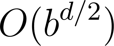 : “explains 84.0% of variance” means
 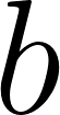 is 0.84.
Three things happened, and each is typical GP behavior:
- GP found the frequency of the oscillator.
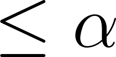
sin(x + x)is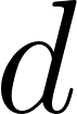 , and notice where the 2 lives: in an addition
  , not a constant multiply. Both spellings cost the same four nodes, but
 x + xneeds no lucky constant, so the search reaches it long before a constant that happens to land near does. It never recovered the damping, because without
 expthe damping factor costs a large tree, and every large tree that might approximatee^{-x/3}lost the parsimony auction to the small one. - Improvement stopped at generation 2 and the population coasted for 37 more generations. Early convergence on a plateau is the normal case, not a bug: tournament selection with
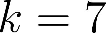 plus elitism consumes diversity quickly. Raise the mutation rate, lower the tournament size, or use the
 targetargument ofevolve()(like examples 2, 3, and 4 do) to stop the waste. - There is no bloat in the final answer (4 nodes!). The parsimony term is small enough not to distort the error comparison (0.0005 per node versus an MSE near 0.09) but large enough that bloated mutants never reproduce.
If you add "exp": (1, lambda a: math.exp(a[0])) to FUNCTIONS, watch the run discover the damping factor. (That is practice problem 1.)
Example 2: Boolean logic synthesis
The canonical GP problem class: evolve a program whose input/output behavior matches a specification. Here the specification is a machine safety interlock. Enable the motor only when both operator keys are turned on, there is no fault signal, and at least one of the two redundant sensors agrees:

The search sees the 32-row truth table and nothing else. Terminals are the five input names plus ephemeral Boolean constants TRUE/FALSE (20% of terminal draws); functions are the three gates AND, OR, NOT. Fitness is the fraction of truth-table rows computed incorrectly, a plain count of wrong behaviors.
Two notes before the listing. First, the constant leaves matter: parity-like and multiplexer-style targets are famously hard for GP without ephemeral constants, because the population spends generations discovering trivial constants. Second, note how little this problem is about syntax: the interlock above has many equivalent netlists, and GP finds one of them, not “the” one.
  1 # Example 2 -- Boolean Logic Synthesis with Tree GP
  2 #
  3 # Genetic programming on the canonical GP problem class: evolve a PROGRAM
  4 # (here, a combinational logic circuit) whose INPUT/OUTPUT behavior matches
  5 # a specification given as a truth table. Fitness counts wrong rows, so the
  6 # landscape is a staircase of partially-correct circuits -- exactly the kind
  7 # of "behavior, not structure" scoring that distinguishes GP from ordinary
  8 # parameter optimization.
  9 #
 10 # The specification is a machine-safety interlock:
 11 #
 12 #   ENABLE = (both operator keys pressed) AND (no fault)
 13 #            AND (at least one of the two redundant sensors agrees)
 14 #
 15 # Inputs: K1, K2 = operator keys; F = fault flag (active high);
 16 #         S1, S2 = redundant sensors. The interlock needs only ONE of the
 17 #         redundant sensors to agree, so the pair is free to disagree on
 18 #         any row and ENABLE still fires.
 19 # Hand-writing the gate netlist for this is error-prone; GP rediscovers a
 20 # correct netlist from 32 example rows in seconds.
 21 #
 22 # This is also a clean illustration of two GP subtleties:
 23 #   * Ephemeral Boolean constants (TRUE/FALSE leaves) -- without them, GP
 24 #     struggles badly on parity-like targets.
 25 #   * Behavior-only scoring: the evolved netlist in our run is NOT the
 26 #     textbook formula. It is a structurally different circuit that
 27 #     computes the same function, and the demo verifies it row by row.
 28 #     GP optimizes what a program DOES, never how it LOOKS.
 29 #
 30 # References:
 31 #   Koza, J. (1992) "Genetic Programming: On the Programming of Computers
 32 #                   by Means of Natural Selection", MIT Press (Boolean
 33 #                   problems)
 34 #   Parity difficulty in GP: Langdon & Poli (1998), "Why Building Blocks
 35 #                   Don't Work on Parity Problems", CSRP-98-17:
 36 #                   http://web4.cs.ucl.ac.uk/staff/W.Langdon/csrp-98-17/eq.html
 37 #   Logic synthesis:           https://en.wikipedia.org/wiki/Logic_synthesis
 38
 39 from __future__ import annotations
 40
 41 import itertools
 42 import random
 43 from collections.abc import Callable, Mapping, Sequence
 44 from typing import Final
 45
 46 from gp_core import (
 47     TerminalSampler,
 48     Tree,
 49     evolve,
 50     mutate_hoist,
 51     mutate_point,
 52     mutate_subtree,
 53     random_tree,
 54 )
 55
 56 SEED: Final = 12
 57
 58 INPUTS: Final[tuple[str, ...]] = ("K1", "K2", "F", "S1", "S2")
 59
 60
 61 def specification(row: Sequence[bool]) -> bool:
 62     """The interlock we want GP to rediscover (row order = INPUTS)."""
 63     k1, k2, fault, s1, s2 = row
 64     return (k1 and k2) and not fault and (s1 or s2)
 65
 66
 67 TRUTH_TABLE: Final[list[tuple[tuple[bool, ...], bool]]] = [
 68     (row, specification(row)) for row in itertools.product((False, True), repeat=len(INPUTS))
 69 ]
 70
 71 # The same cases keyed by input name, built once so fitness() does not
 72 # rebuild a dict for every candidate. Evaluating a tree is the hot path.
 73 CASES: Final[list[tuple[Mapping[str, bool], bool]]] = [
 74     (dict(zip(INPUTS, row, strict=True)), expected) for row, expected in TRUTH_TABLE
 75 ]
 76
 77 # Gate-level function set. NOT is unary; AND/OR binary. (NAND-only synthesis
 78 # is possible too -- try it as an exercise!)
 79 GATES: Final[dict[str, tuple[int, Callable[[Sequence[bool]], bool]]]] = {
 80     "AND": (2, lambda a: a[0] and a[1]),
 81     "OR": (2, lambda a: a[0] or a[1]),
 82     "NOT": (1, lambda a: not a[0]),
 83 }
 84
 85 FUNCTION_ARITIES: Final[dict[str, int]] = {name: arity for name, (arity, _eval) in GATES.items()}
 86
 87
 88 def terminals(rng: random.Random) -> TerminalSampler:
 89     """Inputs plus 20% chance of an Ephemeral Random Boolean constant."""
 90     pool = list(INPUTS)
 91
 92     def sample() -> str:
 93         if rng.random() < 0.2:
 94             return rng.choice(("TRUE", "FALSE"))
 95         return rng.choice(pool)
 96
 97     return sample
 98
 99
100 def evaluate(tree: Tree, row: Mapping[str, bool]) -> bool:
101     """Interpret the tree as a gate netlist over one input row."""
102     if tree.is_leaf:
103         if tree.name == "TRUE":
104             return True
105         if tree.name == "FALSE":
106             return False
107         return row[tree.name]
108     arity, op = GATES[tree.name]
109     if len(tree.args) != arity:
110         return False
111     return op([evaluate(child, row) for child in tree.args])
112
113
114 def fitness(tree: Tree) -> float:
115     """Fraction of truth-table rows the circuit gets WRONG (0.0 = perfect)."""
116     wrong = 0
117     for row, expected in CASES:
118         if evaluate(tree, row) != expected:
119             wrong += 1
120     return float(wrong) / len(CASES)
121
122
123 def render(tree: Tree) -> str:
124     """Human-readable gate expression, e.g. (NOT (K1 AND F))."""
125     if tree.is_leaf:
126         return tree.name
127     arity, _op = GATES[tree.name]
128     kids = [render(child) for child in tree.args]
129     if arity == 2:
130         return f"({kids[0]} {tree.name} {kids[1]})"
131     return f"({tree.name} {kids[0]})"
132
133
134 def build_population(rng: random.Random, size: int, max_depth: int) -> list[Tree]:
135     sampler = terminals(rng)
136     return [
137         random_tree(
138             rng,
139             FUNCTION_ARITIES,
140             sampler,
141             max_depth=max_depth,
142             min_depth=2,
143             method="grow",
144         )
145         for _ in range(size)
146     ]
147
148
149 def main() -> None:
150     rng = random.Random(SEED)
151     population = build_population(rng, size=250, max_depth=8)
152     sampler = terminals(rng)
153
154     def mutate(tree: Tree) -> Tree:
155         roll = rng.random()
156         if roll < 0.45:
157             return mutate_subtree(rng, tree, FUNCTION_ARITIES, sampler, max_depth=4)
158         if roll < 0.9:
159             return mutate_point(rng, tree, FUNCTION_ARITIES, sampler)
160         return mutate_hoist(rng, tree)
161
162     def report(generation: int, best_fitness: float, best: Tree) -> None:
163         print(
164             f"gen {generation:3d}  wrong rows {round(best_fitness * len(CASES)):2d}/32  "
165             f"size {best.size:3d}  {render(best)[:58]}"
166         )
167
168     print("# Evolving a 5-input safety interlock from its 32-row truth table")
169     print("# inputs: K1, K2 (keys), F (fault), S1, S2 (sensors)\n")
170
171     result = evolve(
172         rng,
173         population,
174         fitness,
175         mutate,
176         generations=60,
177         crossover_rate=0.85,
178         mutation_rate=0.12,
179         tournament_size=5,
180         elitism=1,
181         max_depth=12,
182         target=0.0,
183         reporter=report,
184     )
185
186     print(
187         f"\nPerfect circuit found: {result.solved} "
188         f"(generation {result.generations}, {result.best.size} gates, depth {result.best.depth})"
189     )
190     print(f"  ENABLE = {render(result.best)}")
191
192     # Double-check: re-evaluate EVERY row against the discovered netlist.
193     failures = [row for row, expected in CASES if evaluate(result.best, row) != expected]
194     print(f"  verification: {len(CASES) - len(failures)}/{len(CASES)} rows correct")
195
196     print("\n  truth table (1 = ENABLE):")
197     header = "  " + " ".join(f"{name:>2}" for name in INPUTS) + " | spec | evolved"
198     print(header)
199     print("  " + "-" * (len(header) - 2))
200     for row, expected in CASES:
201         got = evaluate(result.best, row)
202         mark = "  " if got == expected else " <-- MISMATCH"
203         bits = " ".join(f"{int(row[name]):>2}" for name in INPUTS)
204         print(f"  {bits} |  {int(expected)}  |   {int(got)}{mark}")
205
206
207 if __name__ == "__main__":
208     main()
Running it
1 make logic # or: uv run python example_2_boolean_logic.py
Output (seed 12):
 1 # Evolving a 5-input safety interlock from its 32-row truth table
 2 # inputs: K1, K2 (keys), F (fault), S1, S2 (sensors)
 3
 4 gen   0  wrong rows  3/32  size   4  (NOT (NOT (NOT TRUE)))
 5 gen   1  wrong rows  2/32  size  28  ((NOT ((F AND S1) OR ((F AND ((NOT K1) OR (S1 OR S2))) OR
 6 gen   2  wrong rows  2/32  size  28  ((NOT ((F AND S1) OR ((F AND ((NOT K1) OR (S1 OR S2))) OR
 7 gen   3  wrong rows  1/32  size  13  (K1 AND ((NOT (F OR (NOT (K2 AND (K1 AND K1))))) AND K1))
 8 gen   4  wrong rows  1/32  size  13  (K1 AND ((NOT (F OR (NOT (K2 AND (K1 AND K1))))) AND K1))
 9 gen   5  wrong rows  1/32  size  13  (K1 AND ((NOT (F OR (NOT (K2 AND (K1 AND K1))))) AND K1))
10 gen   6  wrong rows  1/32  size  13  (K1 AND ((NOT (F OR (NOT (K2 AND (K1 AND K1))))) AND K1))
11 gen   7  wrong rows  1/32  size  13  (K1 AND ((NOT (F OR (NOT (K2 AND (K1 AND K1))))) AND K1))
12 gen   8  wrong rows  0/32  size  18  (((NOT K1) OR (S1 OR S2)) AND ((NOT (F OR (NOT (K2 AND (K2
13
14 Perfect circuit found: True (generation 8, 18 gates, depth 8)
15   ENABLE = (((NOT K1) OR (S1 OR S2)) AND ((NOT (F OR (NOT (K2 AND (K2 AND K1))))) AND K2))
16   verification: 32/32 rows correct
17
18   truth table (1 = ENABLE):
19   K1 K2  F S1 S2 | spec | evolved
20   -------------------------------
21    0  0  0  0  0 |  0  |   0
22    0  0  0  0  1 |  0  |   0
23    0  0  0  1  0 |  0  |   0
24    0  0  0  1  1 |  0  |   0
25    0  0  1  0  0 |  0  |   0
26    0  0  1  0  1 |  0  |   0
27    0  0  1  1  0 |  0  |   0
28    0  0  1  1  1 |  0  |   0
29    0  1  0  0  0 |  0  |   0
30    0  1  0  0  1 |  0  |   0
31    0  1  0  1  0 |  0  |   0
32    0  1  0  1  1 |  0  |   0
33    0  1  1  0  0 |  0  |   0
34    0  1  1  0  1 |  0  |   0
35    0  1  1  1  0 |  0  |   0
36    0  1  1  1  1 |  0  |   0
37    1  0  0  0  0 |  0  |   0
38    1  0  0  0  1 |  0  |   0
39    1  0  0  1  0 |  0  |   0
40    1  0  0  1  1 |  0  |   0
41    1  0  1  0  0 |  0  |   0
42    1  0  1  0  1 |  0  |   0
43    1  0  1  1  0 |  0  |   0
44    1  0  1  1  1 |  0  |   0
45    1  1  0  0  0 |  0  |   0
46    1  1  0  0  1 |  1  |   1
47    1  1  0  1  0 |  1  |   1
48    1  1  0  1  1 |  1  |   1
49    1  1  1  0  0 |  0  |   0
50    1  1  1  0  1 |  0  |   0
51    1  1  1  1  0 |  0  |   0
52    1  1  1  1  1 |  0  |   0
Reading the results
Progress is honest: 3 wrong rows at generation 0 (an always-false constant circuit:  mislabels the 3 rows where the interlock should ENABLE), 2 at generation 1, 1 by generation 3, then a perfect 18-gate circuit at generation 8. The verification line and the printed truth table confirm 32/32 rows.
Compare the evolved netlist with the hand-written formula. They compute the same function, but GP’s answer contains K2 AND (K2 AND K1) where you would write K1 AND K2, and a NOT (F OR (NOT ...)) wrapper that De Morgan’s law collapses into the NOT F you would have written yourself. These are intrinsically redundant subexpressions: code that can never change an output is invisible to selection, so evolution keeps it. If you ship this circuit, you pass it through a Boolean simplifier first. The printed truth table is the point of the whole demo: spec column and evolved column agree on all 32 rows, and GP earned that by behavior, not by deriving anything.
Example 3: Evolving regular expressions
GP is not restricted to numeric programs. The individual here is a pattern program: a tree whose nodes are regex operators (cat, alt, opt, star, plus) and whose leaves are pre-generalized character fragments (D compiles to  ,
, h1 to 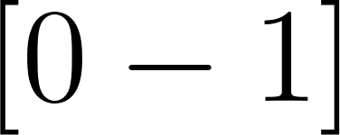 ,
, h3 to 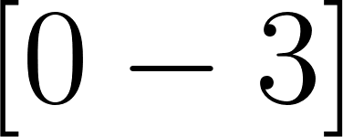 , and so on). Compile the tree to a regex string, run Python’s
 re engine on example strings, score accept/reject.
The task: learn a validator for 24-hour clock times from 8 positive strings and 11 negative strings:
1 positive: 09:15  23:59  00:01  17:42  08:05  12:00  01:30  20:47
2 negative: 24:00  29:00  09:5  9:15  0915  ab:cd  09:60  1:2:3  ''  09:1a  123:45
Nobody tells GP about clock arithmetic. It must discover from misfit pain that hour tens digits live in , that a leading  restricts its follower to , and that minute tens digits live in
 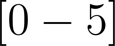 .
.
The fitness function has three parts, and all three earned their place the hard way (see NOTES.md):
- Partial credit on positives. A rejected positive costs
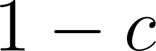 , where
  is the largest fraction of the string the pattern can fully match as a prefix. Patterns that get “23:” or “09:1” right are closer to the truth than patterns that cannot start. This ramp is what lets the search escape the “rejects everything” plateau.
- Full price on false accepts. Accepting any negative costs a flat 1.0, so a pattern that accepts everything stays expensive.
- A never-matching pattern
NEVER_MATCHES$ as a bloat guard. Trees with nested quantifiers or more than quantifier nodes compile to it. This is not cosmetic: Python’s
 reengine backtracks exponentially on patterns like(?:(?:(?:\d*)*)+)*, and one such individual can stall the population evaluation for minutes. We measured this: an unguarded version of this demo hung the machine.
  1 # Example 3 -- Evolving Regular Expressions from String Examples
  2 #
  3 # GP where the "program" is a MATCHER instead of a computer: the evolved
  4 # tree is a pattern program that reads a string and returns accept/reject.
  5 # This flips the usual GP setup in an instructive way -- the phenotype is a
  6 # piece of text-processing logic, the fitness cases are example strings,
  7 # and the primitives are regex operators instead of arithmetic.
  8 #
  9 # Task: synthesize a validator for 24-hour clock times ("09:15", "23:59")
 10 # from POSITIVE and NEGATIVE examples only. Nobody tells GP the structure
 11 # of clock arithmetic; it has to discover that the hour's first digit is
 12 # limited to [0-2], that the minute tens digit is limited to [0-5], and so
 13 # on -- purely from the pain of accepting "24:00" or rejecting "09:15".
 14 #
 15 # Fitness is example-weighted error with a smoothing trick: an unmatched
 16 # positive is charged (1 - best_prefix_fraction) instead of a flat 1.0 --
 17 # how much of the string the pattern could match from the left. Accepting
 18 # a negative still costs a full 1.0, so the search cannot cheat by
 19 # accepting every string, while partial credit stops it from getting
 20 # trapped in plateaus like `(?:(?:[0-2]|:))+` (rejects everything, matches
 21 # almost nothing). A small size term breaks ties toward shorter, cleaner
 22 # patterns.
 23 #
 24 # The terminal alphabet is *pre-generalized*: it contains character-class
 25 # fragments like [0-3] and [4-9] alongside single literals, mimicking how
 26 # real GP-regex tools build patterns from library components.
 27 #
 28 # References:
 29 #   Bartoli, De Lorenzo, Medvet & Tarlao, "Playing Regex Golf with Genetic
 30 #   Programming" (GECCO 2014):
 31 #                   https://doi.org/10.1145/2576768.2598333
 32 #   Bartoli, De Lorenzo, Medvet & Tarlao, "On the Automatic Construction
 33 #   of Regular Expressions from Examples (GP vs. Humans 1-0)" (GECCO
 34 #   2016):          https://doi.org/10.1145/2908961.2930946
 35 #   Python re module:           https://docs.python.org/3/library/re.html
 36
 37 from __future__ import annotations
 38
 39 import functools
 40 import random
 41 import re
 42 from typing import Final
 43
 44 from gp_core import (
 45     TerminalSampler,
 46     Tree,
 47     evolve,
 48     mutate_hoist,
 49     mutate_point,
 50     mutate_subtree,
 51     random_tree,
 52 )
 53
 54 SEED: Final = 1  # chosen so this run converges quickly and repeatably
 55
 56 POSITIVE: Final[list[str]] = [
 57     "09:15",
 58     "23:59",
 59     "00:01",
 60     "17:42",
 61     "08:05",
 62     "12:00",
 63     "01:30",
 64     "20:47",
 65 ]
 66 NEGATIVE: Final[list[str]] = [
 67     "24:00",  # hour out of range
 68     "29:00",  # hour out of range (also punishes [0-5]-for-hours)
 69     "09:5",  # single-digit minutes
 70     "9:15",  # single-digit hour
 71     "0915",  # missing separator
 72     "ab:cd",  # not digits
 73     "09:60",  # minute out of range
 74     "1:2:3",  # extra separator
 75     "",  # empty input
 76     "09:1a",  # non-digit tail
 77     "123:45",  # too many hour digits
 78 ]
 79
 80 # (negative string, cost of accepting it). All equal here; the tuple form
 81 # leaves room to weight near-miss cases differently.
 82 NEGATIVE_WEIGHTS: Final[list[tuple[str, float]]] = [(s, 1.0) for s in NEGATIVE]
 83
 84 # ---------------------------------------------------------------------------
 85 # Pattern-program function set. Every node compiles to a regex fragment;
 86 # unary ops wrap children in (?:...) so precedence is always safe.
 87 # ---------------------------------------------------------------------------
 88
 89 PATTERN_OPS: Final[dict[str, int]] = {
 90     "cat": 2,  # concatenation:  a b
 91     "alt": 2,  # alternation:    a|b
 92     "opt": 1,  # optional:       a?
 93     "star": 1,  # Kleene star:    a*
 94     "plus": 1,  # one-or-more:    a+
 95 }
 96
 97 # The quantifier operators, used by the anti-backtracking guard.
 98 QUANTIFIER_OPS: Final = frozenset({"opt", "star", "plus"})
 99
100 # Terminal alphabet -> regex fragment. Pre-generalized classes do most of
101 # the "cleverness"; GP discovers WHERE they must appear. Deliberately NO
102 # "." wildcard: with prefix credit below, `.` would grant every positive
103 # full credit and flatten the whole fitness landscape into plateaus.
104 TERMINAL_FRAGMENTS: Final[dict[str, str]] = {
105     "D": r"\d",  # any digit
106     "h1": r"[0-1]",  # hour tens digit 0 or 1
107     "h2": r"[0-2]",  # ... alternative tens constraint
108     "h3": r"[0-3]",  # hour units digit when the tens digit is 2
109     "h9": r"[3-9]",  # hour units digit paired with a 0/1 tens digit
110     "m1": r"[0-5]",  # minute tens constraint
111     "m9": r"[6-9]",  # minute tens digit that makes the time invalid
112     "c": r":",  # the separator, as a literal
113     "d0": r"0",
114     "d1": r"1",
115     "d2": r"2",
116     "d5": r"5",
117     "d9": r"9",
118 }
119
120 TERMINAL_POOL: Final[list[str]] = list(TERMINAL_FRAGMENTS)
121
122 FUNCTION_ARITIES: Final[dict[str, int]] = dict(PATTERN_OPS)
123
124 SIZE_PRESSURE: Final = 0.005  # fitness = example error + 0.5% per tree node
125 MAX_QUANTIFIERS: Final = 4  # anti-backtracking guard (see compile_tree)
126 MAX_SOURCE_LEN: Final = 300
127
128 NEVER_MATCHES: Final = r"(?!a)a"  # impossible pattern: fails instantly
129
130
131 def terminals(rng: random.Random) -> TerminalSampler:
132     """Bias leaf sampling toward the meaningful classes, not bare literals."""
133     weights = {"D": 4, "h1": 4, "h2": 3, "h3": 4, "h9": 2, "m1": 4, "m9": 2, "c": 4}
134     pool: list[str] = []
135     for name in TERMINAL_POOL:
136         pool.extend([name] * weights.get(name, 1))
137
138     def sample() -> str:
139         return rng.choice(pool)
140
141     return sample
142
143
144 # ---------------------------------------------------------------------------
145 # Compile a pattern tree into an anchored regex string (and evaluate it).
146 # ---------------------------------------------------------------------------
147
148
149 def quantifier_stats(tree: Tree) -> tuple[int, bool]:
150     """Return (number of quantifier nodes, whether any quantifier nests).
151
152     `nested` is True when a quantifier node has another quantifier anywhere
153     below it, the shape that makes the backtracking `re` engine exponential
154     even on 6-character strings: `(?:(?:(?:[0-5]*)*)+)*` can hang a CPU
155     forever. One post-order pass answers both questions.
156     """
157     total = 1 if tree.name in QUANTIFIER_OPS else 0
158     nested = False
159     for child in tree.args:
160         child_total, child_nested = quantifier_stats(child)
161         total += child_total
162         if child_nested or (tree.name in QUANTIFIER_OPS and child_total):
163             nested = True
164     return total, nested
165
166
167 def compile_tree(tree: Tree) -> str:
168     r"""Tree -> regex source string.
169
170     Bloat guard: trees with more than `MAX_QUANTIFIERS` quantifier nodes,
171     NESTED quantifiers, or an absurdly long source compile to a
172     never-matching pattern. Without this, degenerate candidates like the
173     greedy `(?:\d|:)+` or `(?:(?:[0-5]*)*)+` make fitness evaluation take
174     exponential time on a six-character string -- a dramatic demonstration
175     that fitness evaluation must stay computable. The exact solution here
176     uses no quantifiers at all, so the guard only removes junk.
177
178     The guard is a heuristic, not a proof: a single quantifier over an
179     ambiguous alternation (for example one digit class followed by another)
180     can still backtrack. It is enough because these fitness cases are at
181     most six characters.
182     """
183     count, nested = quantifier_stats(tree)
184     if count > MAX_QUANTIFIERS or nested:
185         return NEVER_MATCHES
186     source = _compile_node(tree)
187     return source if len(source) <= MAX_SOURCE_LEN else NEVER_MATCHES
188
189
190 def _compile_node(tree: Tree) -> str:
191     if tree.is_leaf:
192         return TERMINAL_FRAGMENTS.get(tree.name, re.escape(tree.name))
193     arity = PATTERN_OPS.get(tree.name)
194     if arity is None:  # defensive: unknown function
195         return NEVER_MATCHES
196     kids = [_compile_node(child) for child in tree.args]
197     if len(kids) != arity:  # defensive: malformed tree
198         return NEVER_MATCHES
199     match tree.name:
200         case "cat":
201             return kids[0] + kids[1]
202         case "alt":
203             return f"(?:{kids[0]}|{kids[1]})"
204         case "opt":
205             return f"(?:{kids[0]})?"
206         case "star":
207             return f"(?:{kids[0]})*"
208         case "plus":
209             return f"(?:{kids[0]})+"
210         case _:
211             raise AssertionError(f"unknown pattern op {tree.name!r}")
212
213
214 @functools.lru_cache(maxsize=8192)
215 def compile_cached(source: str) -> re.Pattern[str] | None:
216     """Compile anchored regex text once per distinct string; None if invalid."""
217     try:
218         return re.compile(f"^(?:{source})$")
219     except re.error:
220         return None
221
222
223 def prefix_credit(tree: Tree, text: str) -> float:
224     """Fraction of `text` the pattern can consume from the left (1.0 = match).
225
226     Turns the staircase fitness into a ramp: a pattern that gets half of
227     "23:59" right is closer to the truth than one that cannot even start.
228     Note we must ask "can the WHOLE prefix k be matched?" (fullmatch on
229     text[:k]) -- a plain .match() succeeds as long as the pattern consumes
230     even one character, which would silently grant full credit.
231     """
232     if not text:
233         return 0.0
234     anchored = compile_cached(compile_tree(tree))
235     if anchored is None:
236         return 0.0
237     for k in range(len(text), 0, -1):
238         if anchored.fullmatch(text[:k]):
239             return k / len(text)
240     return 0.0
241
242
243 def matches(tree: Tree, text: str) -> bool:
244     pattern = compile_cached(compile_tree(tree))
245     return pattern is not None and pattern.fullmatch(text) is not None
246
247
248 def fitness(tree: Tree) -> float:
249     r"""Weighted example error + tiny pressure toward short patterns.
250
251     Rejecting a positive costs (1 - prefix_credit); accepting a negative
252     costs its full weight -- see module docstring for why this mix keeps
253     both degenerate strategies (the greedy `(?:\d|:)+` and the
254     never-matching pattern) bad while still giving the search somewhere to
255     climb.
256     """
257     error = 0.0
258     for text in POSITIVE:
259         error += 1.0 - prefix_credit(tree, text)
260     for text, weight in NEGATIVE_WEIGHTS:
261         if matches(tree, text):
262             error += weight
263     return error + SIZE_PRESSURE * tree.size
264
265
266 def render(tree: Tree) -> str:
267     """Pattern source, kept short for progress lines."""
268     text = compile_tree(tree)
269     return text if len(text) <= 58 else text[:55] + "..."
270
271
272 def build_population(rng: random.Random, size: int, max_depth: int) -> list[Tree]:
273     sampler = terminals(rng)
274     return [
275         random_tree(
276             rng,
277             FUNCTION_ARITIES,
278             sampler,
279             max_depth=max_depth,
280             min_depth=3,
281             method="grow",
282         )
283         for _ in range(size)
284     ]
285
286
287 def main() -> None:
288     rng = random.Random(SEED)
289     population = build_population(rng, size=200, max_depth=9)
290     sampler = terminals(rng)
291
292     def mutate(tree: Tree) -> Tree:
293         roll = rng.random()
294         if roll < 0.5:
295             return mutate_subtree(rng, tree, FUNCTION_ARITIES, sampler, max_depth=4)
296         if roll < 0.85:
297             return mutate_point(rng, tree, FUNCTION_ARITIES, sampler)
298         return mutate_hoist(rng, tree)
299
300     def report(generation: int, best_fitness: float, best: Tree) -> None:
301         accepted = sum(1 for s in POSITIVE if matches(best, s))
302         rejected = sum(1 for s, _w in NEGATIVE_WEIGHTS if not matches(best, s))
303         print(
304             f"gen {generation:3d}  fit {best_fitness:6.3f}  "
305             f"pos {accepted}/{len(POSITIVE)}  neg {rejected}/{len(NEGATIVE)}  {render(best)[:40]}"
306         )
307
308     print("# Evolving a regular expression for 24-hour clock times")
309     print(f"# {len(POSITIVE)} positive, {len(NEGATIVE)} negative example strings\n")
310
311     result = evolve(
312         rng,
313         population,
314         fitness,
315         mutate,
316         generations=100,
317         crossover_rate=0.85,
318         mutation_rate=0.12,
319         tournament_size=5,
320         elitism=2,
321         max_depth=12,
322         target=SIZE_PRESSURE * 20,  # zero example error with <= 20 nodes
323         reporter=report,
324     )
325
326     best_source = compile_tree(result.best)
327     print(f"\nEvolved pattern ({result.best.size} nodes, depth {result.best.depth}):")
328     print(f"  ^{best_source}$")
329     print(f"  all examples satisfied: {result.solved}")
330
331     print("\n  input       expected  evolved")
332     for text in POSITIVE:
333         print(f"  {text:<10}  MATCH     {'MATCH' if matches(result.best, text) else 'no match'}")
334     for text in NEGATIVE:
335         shown = text if text else "<empty>"
336         verdict = "REJECTED" if not matches(result.best, text) else "accepted (!)"
337         print(f"  {shown:<10}  reject    {verdict}")
338
339     # Show generalization: strings the GP system never saw.
340     print("\n  unseen probes:")
341     for text in ["05:59", "23:61", "22:00", "07:7", "11:11", "2:03"]:
342         verdict = "MATCH" if matches(result.best, text) else "reject"
343         truth = "valid" if re.fullmatch(r"([01]\d|2[0-3]):[0-5]\d", text) else "invalid"
344         print(f"  {text:<8} -> {verdict:<7} ({truth})")
345
346
347 if __name__ == "__main__":
348     main()
Running it
1 make regex # or: uv run python example_3_regex_synthesis.py
Output (seed 1):
 1 # Evolving a regular expression for 24-hour clock times
 2 # 8 positive, 11 negative example strings
 3
 4 gen   0  fit  5.430  pos 0/8  neg 11/11  (?:9[3-9]|(?:[0-3])+)
 5 gen   1  fit  5.410  pos 0/8  neg 11/11  (?:[0-3])+
 6 gen   2  fit  4.830  pos 0/8  neg 11/11  (?:[0-3][3-9]|(?:[0-3])+)
 7 gen   3  fit  4.830  pos 0/8  neg 11/11  (?:[0-3][3-9]|(?:[0-3])+)
 8 gen   4  fit  4.830  pos 0/8  neg 11/11  (?:[0-3][3-9]|(?:[0-3])+)
 9 gen   5  fit  4.830  pos 0/8  neg 11/11  (?:[0-3][3-9]|(?:[0-3])+)
10 gen   6  fit  4.830  pos 0/8  neg 11/11  (?:[0-3][3-9]|(?:[0-3])+)
11 gen   7  fit  4.830  pos 0/8  neg 11/11  (?:[0-3][3-9]|(?:[0-3])+)
12 gen   8  fit  4.830  pos 0/8  neg 11/11  (?:[0-3][3-9]|(?:[0-3])+)
13 gen   9  fit  4.830  pos 0/8  neg 11/11  (?:[0-3][3-9]|(?:[0-3])+)
14 gen  10  fit  4.830  pos 0/8  neg 11/11  (?:[0-3][3-9]|(?:[0-3])+)
15 gen  11  fit  4.830  pos 0/8  neg 11/11  (?:[0-3][3-9]|(?:[0-3])+)
16 gen  12  fit  4.830  pos 0/8  neg 11/11  (?:[0-3][3-9]|(?:[0-3])+)
17 gen  13  fit  4.830  pos 0/8  neg 11/11  (?:[0-3][3-9]|(?:[0-3])+)
18 gen  14  fit  4.830  pos 0/8  neg 11/11  (?:[0-3][3-9]|(?:[0-3])+)
19 gen  15  fit  4.830  pos 0/8  neg 11/11  (?:[0-3][3-9]|(?:[0-3])+)
20 gen  16  fit  4.830  pos 0/8  neg 11/11  (?:[0-3][3-9]|(?:[0-3])+)
21 gen  17  fit  4.070  pos 0/8  neg 11/11  (?:[0-3][3-9]|(?:(?:5:)+|[0-1]\d:))
22 gen  18  fit  3.680  pos 0/8  neg 11/11  (?:[0-3][3-9]|(?:(?:[0-3][3-9]|(?:[0-3])
23 gen  19  fit  3.270  pos 0/8  neg 11/11  (?:[0-3][3-9]|(?:(?:5:)+|[0-5]\d:))
24 gen  20  fit  3.260  pos 0/8  neg 11/11  (?:(?:[0-3][3-9]|(?:[0-3])+)(?::)+|(?:[0
25 gen  21  fit  2.730  pos 0/8  neg 11/11  (?:[0-3](?:[0-3](?::)+|:)[3-9]|(?:(?:5:)
26 gen  22  fit  2.730  pos 0/8  neg 11/11  (?:[0-3](?:[0-3](?::)+|:)[3-9]|(?:(?:5:)
27 gen  23  fit  2.720  pos 0/8  neg 11/11  (?:[0-3](?:[0-3](?::)+|:)[3-9]|(?:(?:[0-
28 gen  24  fit  2.350  pos 0/8  neg 11/11  (?:(?:[0-3](?:[0-3](?::)+|[0-3])|(?:[0-3
29 gen  25  fit  1.755  pos 3/8  neg 11/11  (?:(?:[0-3](?:[0-3](?::)+|[0-3])|(?:[0-3
30 gen  26  fit  1.755  pos 3/8  neg 11/11  (?:(?:[0-3](?:[0-3](?::)+|[0-3])|(?:[0-3
31 gen  27  fit  1.755  pos 3/8  neg 11/11  (?:(?:[0-3](?:[0-3](?::)+|[0-3])|(?:[0-3
32 gen  28  fit  1.190  pos 8/8  neg 10/11  (?:[0-1]\d:(?:[0-5])+|(?:(?:(?:[0-3](?:[
33 gen  29  fit  1.170  pos 8/8  neg 10/11  (?:[0-1]\d:(?:[0-5])+|(?:(?:(?:[0-3](?:[
34 gen  30  fit  1.170  pos 8/8  neg 10/11  (?:[0-1]\d:(?:[0-5])+|(?:(?:(?:[0-3](?:[
35 gen  31  fit  1.170  pos 8/8  neg 10/11  (?:[0-1]\d:(?:[0-5])+|(?:(?:(?:[0-3](?:[
36 gen  32  fit  1.165  pos 8/8  neg 10/11  (?:[0-1]\d:(?:[0-5])+|(?:(?:(?:[0-3](?:[
37 gen  33  fit  1.135  pos 8/8  neg 10/11  (?:[0-1]\d:(?:[0-5])+|(?:(?:[0-3](?:[0-3
38 gen  34  fit  1.135  pos 8/8  neg 10/11  (?:[0-1]\d:(?:[0-5])+|(?:(?:[0-3](?:[0-3
39 gen  35  fit  1.125  pos 8/8  neg 10/11  (?:[0-1]\d:(?:[0-5])+|(?:(?:[0-3](?:[0-3
40 gen  36  fit  0.140  pos 8/8  neg 11/11  (?:[0-1]\d:(?:[0-5])+(?:[0-5])+|(?:(?:[0
41 gen  37  fit  0.140  pos 8/8  neg 11/11  (?:[0-1]\d:(?:[0-5])+(?:[0-5])+|(?:(?:[0
42 gen  38  fit  0.130  pos 8/8  neg 11/11  (?:[0-1]\d:(?:[0-5])+(?:[0-5])+|(?:[0-3]
43 gen  39  fit  0.130  pos 8/8  neg 11/11  (?:[0-1]\d:(?:[0-5])+(?:[0-5])+|(?:[0-3]
44 gen  40  fit  0.125  pos 8/8  neg 11/11  (?:[0-1]\d:[0-5](?:[0-5])+|(?:[0-3](?:[0
45 gen  41  fit  0.120  pos 8/8  neg 11/11  (?:[0-1]\d:[0-5](?:[0-5])+|(?:(?:[0-3]\d
46 gen  42  fit  0.120  pos 8/8  neg 11/11  (?:[0-1]\d:[0-5](?:[0-5])+|(?:(?:[0-3]\d
47 gen  43  fit  0.120  pos 8/8  neg 11/11  (?:[0-1]\d:[0-5](?:[0-5])+|(?:(?:[0-3]\d
48 gen  44  fit  0.105  pos 8/8  neg 11/11  (?:[0-1]\d:[0-5][0-5]|(?:[0-3]\d:|[0-5])
49 gen  45  fit  0.105  pos 8/8  neg 11/11  (?:[0-1]\d:[0-5][0-5]|(?:[0-3]\d:|[0-5])
50 gen  46  fit  0.105  pos 8/8  neg 11/11  (?:[0-1]\d:[0-5][0-5]|(?:[0-3]\d:|[0-5])
51 gen  47  fit  0.105  pos 8/8  neg 11/11  (?:[0-1]\d:[0-5][0-5]|(?:[0-3]\d:|[0-5])
52 gen  48  fit  0.095  pos 8/8  neg 11/11  (?:[0-1]\d:[0-5][0-5]|[0-3]\d:\d[3-9])
53
54 Evolved pattern (19 nodes, depth 6):
55   ^(?:[0-1]\d:[0-5][0-5]|[0-3]\d:\d[3-9])$
56   all examples satisfied: True
57
58   input       expected  evolved
59   09:15       MATCH     MATCH
60   23:59       MATCH     MATCH
61   00:01       MATCH     MATCH
62   17:42       MATCH     MATCH
63   08:05       MATCH     MATCH
64   12:00       MATCH     MATCH
65   01:30       MATCH     MATCH
66   20:47       MATCH     MATCH
67   24:00       reject    REJECTED
68   29:00       reject    REJECTED
69   09:5        reject    REJECTED
70   9:15        reject    REJECTED
71   0915        reject    REJECTED
72   ab:cd       reject    REJECTED
73   09:60       reject    REJECTED
74   1:2:3       reject    REJECTED
75   <empty>     reject    REJECTED
76   09:1a       reject    REJECTED
77   123:45      reject    REJECTED
78
79   unseen probes:
80   05:59    -> MATCH   (valid)
81   23:61    -> reject  (invalid)
82   22:00    -> reject  (valid)
83   07:7     -> reject  (invalid)
84   11:11    -> MATCH   (valid)
85   2:03     -> reject  (invalid)
Reading the results
Read the progress log as a story of discovery. For twenty generations the population only builds hour-fraction fragments ( ,
, 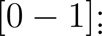 ) because partial credit pays for prefixes. At generation 25 the best pattern already accepts 3 of 8 positives. At generation 36 it accepts all 8 positives and rejects all 11 negatives, and the rest of the run is pure size pressure deleting wrapper nodes (
 simplifies toward
  ).
).
The final answer deserves a close look:
1 ^(?:[0-1]\d:[0-5][0-5]|[0-3]\d:\d[3-9])$
It is not the textbook regex  . The first branch is textbook-like (
 hours, minutes). The second branch handles the
 2-o’clock hours in a way a human would not write: 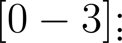 for the hours, followed by
 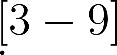 for the minutes. Why is that correct on all examples? It never has to be “the minutes rule”. It only has to reject
 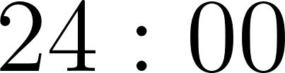 and
and 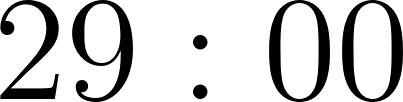 while accepting
 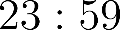 . Pairing “hours in
 [0-3]\d” with “minute units in [3-9]$” does exactly that on this example set, and the two branches together cover all eight positives. It satisfies the specification-as-examples. It is also wrong about clock times in general, and the unseen-probes section prints the confession: 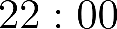 is a valid time that this pattern rejects.
That is the overfitting lesson of this chapter, delivered automatically: GP searched until the fitness cases were exhausted, and the fitness cases were all it ever saw. More negative examples ( as a positive would have done it) or a held-out validation set are the standard cures.
Example 4: Evolving plant growth rules
The last example evolves the most “program-like” individuals yet: L-system growth rules, judged by the organisms they grow. An L-system rewrites a string iteratively; here the rule is F -> (something), applied four times starting from the axiom F, and the final string is read by a turtle:
1 F  move forward, drawing a segment
2 f  move forward WITHOUT drawing
3 +  turn left 25 degrees     -  turn right 25 degrees
4 [  push position and heading    ]  pop them back  (a branch)
A GP tree, say seq(F, branch(seq(+, F))), renders to the rule text F[+F]. Apply it, draw it, and compare the painted cells against a target plant grown from a hidden rule. Fitness is the Jaccard distance between the two cell sets:
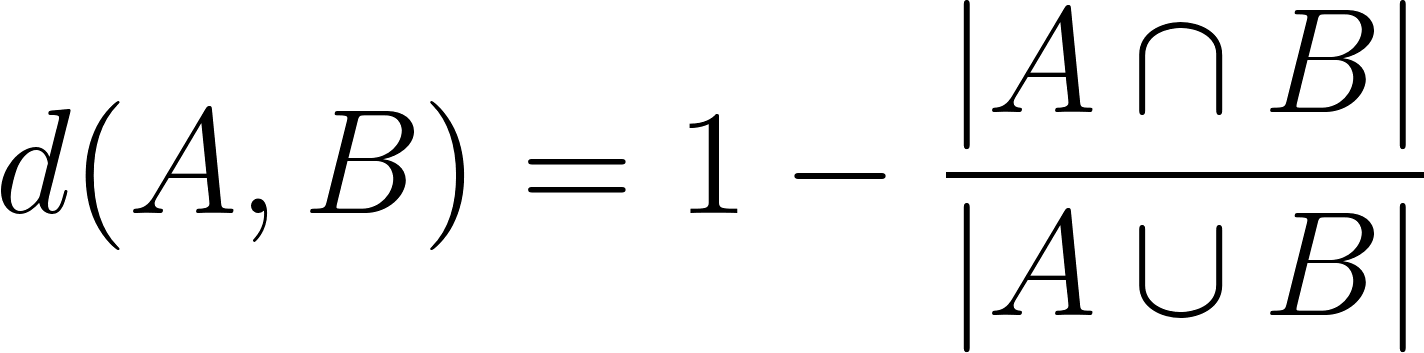
with 0.0 meaning pixel-perfect and larger values meaning less overlap. Every candidate paints the shared start cell, so the distance never quite reaches 1.0.
This demo shows the genotype-phenotype distinction more sharply than the other three. The genotype is a small rule tree (the winner below uses 25 nodes); the phenotype is a plant built from a string of thousands of characters grown by iterating one rule four times. Selection never touches the string; it only sees the cells.
One tuning lesson, recorded in NOTES.md: with five rewrite iterations every candidate plant saturates the grid into a dense blob, the Jaccard score stops discriminating, and runs plateau around 0.34 forever. Four iterations keep the target sparse and the landscape informative. When a GP run “cannot improve,” check whether the fitness function still distinguishes good from better.
  1 # Example 4 -- Evolving L-System Growth Rules to Match a Target Plant
  2 #
  3 # GP where the evolved object is a BIOLOGICAL DEVELOPMENT PROGRAM: an
  4 # L-system rule whose repeated application grows a plant, and whose fitness
  5 # is the plant's shape. This is the most "developmental" of the four demos --
  6 # a tiny genotype (the rule tree) unfolds into a large phenotype (the
  7 # rendered plant) through iterative rewriting, exactly as genes unfold
  8 # into organisms.
  9 #
 10 # Task: we show GP a target plant -- grown by a known rule we keep secret --
 11 # and evolve replacement rules F -> ... until the evolved plant's occupied
 12 # cells overlap the target's cells. The fitness is the JACCARD DISTANCE of
 13 # the two cell sets: 0.0 means "pixel-perfect" and higher is worse. Every
 14 # candidate paints the shared start cell, so the distance stays below 1.0.
 15 # Because every candidate is rendered to the same grid, the landscape is
 16 # surprisingly smooth: rules that grow "taller, then bushier, then leaning
 17 # left" climb the fitness staircase gradually.
 18 #
 19 # Turtle semantics (classic L-system drawing):
 20 #   F  move forward, drawing a segment
 21 #   f  move forward WITHOUT drawing (a stem you cannot see)
 22 #   +  turn left 25 degrees        -  turn right 25 degrees
 23 #   [ push position+heading         ]  pop them back (a branch!)
 24 #
 25 # References:
 26 #   L-systems:       https://en.wikipedia.org/wiki/L-system
 27 #   Prusinkiewicz & Lindenmayer, "The Algorithmic Beauty of Plants"
 28 #   Jacob, C. (1994) "Genetic L-System Programming", PPSN III:
 29 #                    https://doi.org/10.1007/3-540-58484-6_277
 30
 31 from __future__ import annotations
 32
 33 import math
 34 import random
 35 from typing import Final
 36
 37 from gp_core import (
 38     TerminalSampler,
 39     Tree,
 40     evolve,
 41     mutate_hoist,
 42     mutate_point,
 43     mutate_subtree,
 44     random_tree,
 45 )
 46
 47 SEED: Final = 42
 48 GRID_W: Final = 61
 49 GRID_H: Final = 31
 50 ITERATIONS: Final = 4
 51 MAX_EXPANSION: Final = 12000  # rewrite length cap (anti-explosion guard)
 52 TURN_DEG: Final = 25.0
 53
 54 # Rule-grammar function set: seq glues tokens, branch wraps in [ ].
 55 FUNCTION_ARITIES: Final[dict[str, int]] = {"seq": 2, "branch": 1}
 56
 57 # Turtle alphabet as terminals. 'branch'/'seq' are the only nonterminals.
 58 TERMINAL_POOL: Final[list[str]] = ["F", "F", "F", "f", "+", "-"]
 59
 60
 61 def terminals(rng: random.Random) -> TerminalSampler:
 62     pool = list(TERMINAL_POOL)
 63
 64     def sample() -> str:
 65         return rng.choice(pool)
 66
 67     return sample
 68
 69
 70 # ---------------------------------------------------------------------------
 71 # Genotype -> phenotype: expand the rule tree, rewrite the axiom, draw.
 72 # ---------------------------------------------------------------------------
 73
 74
 75 def rule_text(tree: Tree) -> str:
 76     """Render a rule tree as L-system RHS text, e.g. F[+F][-F]F."""
 77     if tree.is_leaf:
 78         return tree.name
 79     kids = [rule_text(child) for child in tree.args]
 80     if tree.name == "seq":
 81         return kids[0] + kids[1]
 82     return f"[{kids[0]}]"
 83
 84
 85 def expand(rule: str, iterations: int = ITERATIONS) -> str:
 86     """Apply `F -> rule` to every F, `iterations` times, from axiom F."""
 87     string = "F"
 88     for _ in range(iterations):
 89         string = string.replace("F", rule)
 90         if len(string) > MAX_EXPANSION:
 91             return string[:MAX_EXPANSION]
 92     return string
 93
 94
 95 def render_grid(string: str) -> set[tuple[int, int]]:
 96     """Turtle-walk an L-system string; return the set of painted cells."""
 97     x = GRID_W // 2.0
 98     y = GRID_H - 1.0
 99     heading = 90.0  # pointing up
100     stack: list[tuple[float, float, float]] = []
101     cells: set[tuple[int, int]] = {(int(round(x)), int(round(y)))}
102
103     for token in string:
104         if token == "F":
105             angle = math.radians(heading)
106             x += math.cos(angle)
107             y -= math.sin(angle)  # image rows grow downward
108             cell = (int(round(x)), int(round(y)))
109             if 0 <= cell[0] < GRID_W and 0 <= cell[1] < GRID_H:
110                 cells.add(cell)
111         elif token == "f":
112             angle = math.radians(heading)
113             x += math.cos(angle)
114             y -= math.sin(angle)
115         elif token == "+":
116             heading += TURN_DEG
117         elif token == "-":
118             heading -= TURN_DEG
119         elif token == "[":
120             stack.append((x, y, heading))
121         elif token == "]" and stack:
122             x, y, heading = stack.pop()
123     return cells
124
125
126 # The hidden target plant: grown from a rule GP must rediscover.
127 TARGET_RULE: Final = "F[+F]F[-F]F"
128 TARGET_CELLS: Final[set[tuple[int, int]]] = render_grid(expand(TARGET_RULE))
129
130
131 def jaccard_distance(tree: Tree) -> float:
132     """1 - |overlap| / |union| of painted cells against the target plant.
133
134     The turtle always paints its start cell, so both sets are non-empty and
135     the result is 0.0 for a pixel-perfect plant.
136     """
137     cells = render_grid(expand(rule_text(tree)))
138     union = len(cells | TARGET_CELLS)
139     return 1.0 - len(cells & TARGET_CELLS) / union
140
141
142 def print_plant(cells: set[tuple[int, int]], label: str) -> None:
143     """Print one plant as an ASCII grid under a heading."""
144     print(f"\n{label}")
145     for row in range(GRID_H):
146         print("  " + "".join("#" if (col, row) in cells else "." for col in range(GRID_W)))
147
148
149 def build_population(rng: random.Random, size: int, max_depth: int) -> list[Tree]:
150     sampler = terminals(rng)
151     return [
152         random_tree(
153             rng,
154             FUNCTION_ARITIES,
155             sampler,
156             max_depth=max_depth,
157             min_depth=2,
158             method="grow",
159         )
160         for _ in range(size)
161     ]
162
163
164 def main() -> None:
165     rng = random.Random(SEED)
166     population = build_population(rng, size=300, max_depth=7)
167     sampler = terminals(rng)
168
169     def mutate(tree: Tree) -> Tree:
170         roll = rng.random()
171         if roll < 0.5:
172             return mutate_subtree(rng, tree, FUNCTION_ARITIES, sampler, max_depth=3)
173         if roll < 0.85:
174             return mutate_point(rng, tree, FUNCTION_ARITIES, sampler)
175         return mutate_hoist(rng, tree)
176
177     def report(generation: int, best_fitness: float, best: Tree) -> None:
178         print(f"gen {generation:3d}  jaccard {best_fitness:6.3f}  rule F -> {rule_text(best)[:30]}")
179
180     print("# Evolving an L-system growth rule to reproduce a target plant")
181     print(f"# grid {GRID_W}x{GRID_H}, {ITERATIONS} rewrite iterations, turn {TURN_DEG:.0f} deg\n")
182
183     result = evolve(
184         rng,
185         population,
186         jaccard_distance,
187         mutate,
188         generations=70,
189         crossover_rate=0.85,
190         mutation_rate=0.12,
191         tournament_size=6,
192         elitism=2,
193         max_depth=10,
194         target=0.02,
195         reporter=report,
196     )
197
198     print(f"\nsecret target rule was:  F -> {TARGET_RULE}")
199     print(f"evolved rule:            F -> {rule_text(result.best)}")
200     print(
201         f"shape distance {result.best_fitness:.3f} after {result.generations} generations "
202         f"(pixel-perfect: {result.best_fitness == 0.0})"
203     )
204
205     print_plant(TARGET_CELLS, "TARGET PLANT (the hidden rule's phenotype):")
206     print_plant(render_grid(expand(rule_text(result.best))), "EVOLVED PLANT (GP's rule phenotype):")
207
208
209 if __name__ == "__main__":
210     main()
Running it
1 make plants # or: uv run python example_4_lsystem_plants.py
Output (seed 42), including both ASCII-art plants:
 1 # Evolving an L-system growth rule to reproduce a target plant
 2 # grid 61x31, 4 rewrite iterations, turn 25 deg
 3
 4 gen   0  jaccard  0.608  rule F -> [FF[f]]fF[F]FFF
 5 gen   1  jaccard  0.538  rule F -> [[[F]]]F[[f]][[F]]FF[f][-FFF]
 6 gen   2  jaccard  0.538  rule F -> [[[F]]]F[[f]][[F]]FF[f][-FFF]
 7 gen   3  jaccard  0.537  rule F -> [[[[F]F]]]F[FfF]FF[-F[F]]
 8 gen   4  jaccard  0.537  rule F -> [[[[F]F]]]F[FfF]FF[-F[F]]
 9 gen   5  jaccard  0.467  rule F -> [[[F]]]F[[f]][F]FF[f][F[[f]][[
10 gen   6  jaccard  0.467  rule F -> [[[F]]]F[[f]][F]FF[f][F[[f]][[
11 gen   7  jaccard  0.458  rule F -> [F+F]F[FfF]FF[-F[F]]
12 gen   8  jaccard  0.458  rule F -> [F+F]F[FfF]FF[-F[F]]
13 gen   9  jaccard  0.432  rule F -> [F+F]F[Ff[+]]FF[-[F]]
14 gen  10  jaccard  0.395  rule F -> [F+F]F[Ff[+]]FF[[[F]]]
15 gen  11  jaccard  0.160  rule F -> [F+F]F[F-F]FF[f[F]]
16 gen  12  jaccard  0.160  rule F -> [F+F]F[F-F]FF[f[F]]
17 gen  13  jaccard  0.000  rule F -> [F+F]F[F-F]FF[f[+]]
18
19 secret target rule was:  F -> F[+F]F[-F]F
20 evolved rule:            F -> [F+F]F[F-F]FF[f[+]]
21 shape distance 0.000 after 13 generations (pixel-perfect: True)
22
23 TARGET PLANT (the hidden rule's phenotype):
24   ............................###..............................
25   .............................##..............................
26   ..............................#..............................
27   ..............................##.............................
28   ..............................###.#..........................
29   ..............................#..###.........................
30   .............................#####...........................
31   .............................#####...........................
32   ..............................###............................
33   ..............................##.............................
34   ..............................###............................
35   ..............................#..............................
36   ..............................##.............................
37   ..........................###.###............................
38   ..........................##..#..............................
39   ...........................####..............................
40   ..........................#####..............................
41   ...........................##.#..............................
42   ............................###..............................
43   .............................##..............................
44   ..............................#..............................
45   ..............................##.............................
46   ..............................###............................
47   ..............................#..............................
48   .............................##..............................
49   .............................##..............................
50   ..............................#..............................
51   ..............................#..............................
52   ..............................#..............................
53   ..............................#..............................
54   ..............................#..............................
55
56 EVOLVED PLANT (GP's rule phenotype):
57   ............................###..............................
58   .............................##..............................
59   ..............................#..............................
60   ..............................##.............................
61   ..............................###.#..........................
62   ..............................#..###.........................
63   .............................#####...........................
64   .............................#####...........................
65   ..............................###............................
66   ..............................##.............................
67   ..............................###............................
68   ..............................#..............................
69   ..............................##.............................
70   ..........................###.###............................
71   ..........................##..#..............................
72   ...........................####..............................
73   ..........................#####..............................
74   ...........................##.#..............................
75   ............................###..............................
76   .............................##..............................
77   ..............................#..............................
78   ..............................##.............................
79   ..............................###............................
80   ..............................#..............................
81   .............................##..............................
82   .............................##..............................
83   ..............................#..............................
84   ..............................#..............................
85   ..............................#..............................
86   ..............................#..............................
87   ..............................#..............................
Reading the results
The run goes 0.608 to 0.537 to 0.467 to 0.395, then 0.160 at generation 11, then 0.000 at generation 13: thirteen generations, a few thousand evaluated plants, one perfect plant. Look at the two rules:
1 secret target rule: F -> F[+F]F[-F]F
2 evolved rule:       F -> [F+F]F[F-F]FF[f[+]]
They are not the same rule. They grow the same set of cells on this grid. The turtle’s world is 61 by 31 integer cells and a plain  step and an inside a pushed branch can land on identical cells when the turn angles are small; the evolved rule’s trailing
  pushes an invisible stub that paints nothing. Both plants therefore have the same phenotype. The final lines print both grids so you can verify the claim yourself.
This is why GP papers insist on behavioral fitness evaluation and on validation examples: scoring the genotype (the rule text) would be a string-edit metric with no relationship to the plants, and scoring behavior on one example plant (as we do) is perfect only up to equivalence classes GP never sees through.
The wider family of GP methods
Tree GP is the original form and still the most common, but it is one member of a family. Most variants exist to fix a specific weakness of plain tree GP, and knowing which one to reach for saves a lot of wasted tuning.
| Variant | Idea | Fixes |
|---|---|---|
| Tree GP | programs are expression trees (this chapter) | the baseline |
| Strongly typed GP | every node has a type, and crossover respects it | mixing numbers, Booleans, and other types |
| Linear GP | programs are sequences of register-machine instructions | faster evaluation, easier constants |
| Grammatical evolution | a list of integers is mapped through a grammar | guarantees syntax, supports any grammar |
| Gene expression programming | a fixed-length chromosome decodes to expression trees | keeps a simple genome, gains tree flexibility |
| Cartesian GP | programs are graphs of indexed nodes | circuits, neural networks, reusable structure |
| PushGP | programs are stack code in a typed language | multiple data types, self-modifying programs |
| Semantic GP | operators act on program behavior, not syntax | smoother landscapes for regression |
| Multi-objective GP | optimizes accuracy and size together | principled bloat control |
| Island and age-layered models | subpopulations exchange migrants, or ages are layered | premature convergence and diversity loss |
A few of these deserve one sentence each:
- Strongly typed GP (Montana, 1995) gives every node a type. Crossover only swaps subtrees of compatible types, so a Boolean can never be dropped into a numeric argument. If you want to evolve a program that mixes numbers, Booleans, and sequences, this is the variant you want.
- Linear GP (Nordin, 1994) represents a program as a sequence of instructions for a simple register machine. Evaluation is a fast loop over a list, and constants are easier to handle than they are in trees.
- Grammatical evolution (Ryan, Collins and O’Neill, 1998) keeps a fixed-length list of integers as the genotype and uses it to choose production rules from a grammar. The grammar guarantees that every decoded program is syntactically valid, which is a strong advantage when the target language has a strict syntax.
- Gene expression programming (Ferreira, 2001) uses a fixed-length chromosome that decodes into expression trees, combining a simple genome with tree-shaped programs.
- Cartesian GP (Miller and Thomson, 2000) evolves a directed graph of indexed nodes. It is a natural fit for circuits and neural networks, where reuse and fan-out matter more than tree structure.
- PushGP (Spector and Robinson, 2002) evolves stack programs in the Push language, which supports several data types and even self-modifying code. It has produced strong results on program synthesis benchmarks.
- Semantic and geometric semantic GP (Moraglio, Krawiec and Johnson, 2012) define operators that act on the vector of program outputs rather than on syntax. For regression problems this turns a rugged landscape into a smoother one and can speed convergence dramatically.
- Multi-objective GP uses a Pareto-based algorithm such as NSGA-II (Deb et al., 2002) to keep a front of accuracy-versus-size trade-offs, which is a cleaner way to control bloat than a hand-tuned penalty.
- Island models and age-layered populations (ALPS, Hornby, 2006) split the population into subpopulations that exchange a few migrants, or protect young individuals from competition with older ones. Both slow premature convergence and are standard in long runs.
There are also hybrids. Memetic GP runs a local optimizer on the constants inside each tree. GP can seed a neural network’s architecture, or a neural network can guide GP’s operator choice. And a large language model can now propose an initial population or a function set for GP to optimize, which combines the model’s broad prior knowledge with GP’s exact, measurable search.
What GP is good at, and when not to reach for it
GP is not a general replacement for machine learning. It is a specific tool for a specific situation, and it pays to know which situation you are in.
Where GP shines
- The structure is unknown. You can write down the inputs, the outputs, and a way to score a candidate, but not the model.
- You can simulate the objective. A physics engine, a circuit simulator, a parser, or a game gives you a behavioral score with no gradient.
- The answer must be readable. A short formula, a gate netlist, or a regex can be reviewed by a domain expert in a way that a weight matrix cannot.
- Data is scarce. GP can work from a small set of examples or a simulator, and it does not need millions of labeled points.
- You want several good answers. A population gives you a set of diverse solutions, not one point estimate, which is useful when the final choice involves constraints the fitness did not encode.
- A few million evaluations are affordable. That is the realistic currency of a GP run.
Where GP struggles
- Gradients are cheap. If backpropagation or least squares applies, use it. GP will be slower and less accurate.
- Fitness is very expensive or very noisy. Every candidate costs an evaluation, so a fitness function that takes minutes or returns a different answer each time is a serious obstacle. Surrogate models and averaging help, but only so much.
- The landscape is deceptive. Parity is the standard example: the fraction of correct rows gives almost no signal until the program is nearly complete, so search is closer to guessing. Example 2 discusses this.
- You need guarantees. GP is a stochastic search with no correctness proof. Safety-critical logic needs formal verification on top of whatever GP proposes.
- The solution needs long-range coordination. Problems where many parts must be right simultaneously, with no partial credit, are hard for any local search.
- You cannot afford to repeat the run. A single lucky seed is not evidence. If you cannot afford dozens of runs, you cannot say much about the method’s reliability.
GP and its neighbors, honestly
- Versus neural networks. Use networks for perception, high-dimensional input, and abundant data. Use GP for structure discovery, small data, and interpretable output. The two are complementary: a network can be a component inside a GP tree, or a fitness predictor.
- Versus reinforcement learning. Reinforcement learning handles sequential decisions with delayed reward. GP can evolve a policy or a controller too, and it is often simpler when the policy can be written as a program and episodes are cheap.
- Versus program synthesis. Constraint solvers and sketch-based synthesis are exact and fast when you have a formal specification. GP works from examples and a score, which is weaker but applies when no formal specification exists.
- Versus a large language model. A language model proposes code from a description; GP optimizes code against measurements. Neither subsumes the other. Use the model to write candidate programs, the function set, or the test cases, and use GP to search the space the model suggests.
A note on stochasticity
GP is a randomized search. One run that finds a good answer proves very little, and one run that fails proves even less. Report the median and the spread over at least a few dozen seeds, and look at the best-so-far curves rather than only the final number. Every demo in this chapter takes a SEED constant for exactly this reason; changing it is the first experiment you should run.
GP in the real world
GP has been applied wherever a program can be scored. A short gallery of the areas where it has earned its keep:
- Symbolic regression and scientific discovery. The oldest application is fitting a formula to data. Schmidt and Lipson’s 2009 result went further and recovered conservation laws and equations of motion from sensor data with no model supplied in advance. Symbolic regression is now used in physics, chemistry, biology, and engineering to turn measurements into interpretable equations.
- Circuit design and evolvable hardware. Koza’s group evolved analog circuits that were patented as genuinely new designs, and GP has been used for filters, amplifiers, and digital logic. In the 1990s Adrian Thompson evolved a configuration for a field-programmable gate array that discriminated tones without a clock, exploiting the physical quirks of the chip in ways a human designer would not have tried.
- Antenna design. Researchers at NASA used genetic programming to design spacecraft antennas with unusual shapes that met their performance specifications and flew on missions. This is a good example of a fitness function that is a physics simulation and a result that is a physical object.
- Robot controllers and behavior. GP can evolve a control program directly from a simulated robot’s behavior, including walking gaits and navigation strategies. The fitness is the simulation, so no dynamics model needs to be differentiable.
- Games and game AI. Evolving heuristics and opponent strategies for board games and video games, and generating content such as levels or rules.
- Scheduling, routing, and logistics. Job-shop scheduling, vehicle routing, and resource allocation, where the evolved program is a dispatch rule.
- Image and signal processing. Evolving filters, feature extractors, and small classifiers, often as a preprocessing step in front of a conventional learner.
- Medicine and biology. Classifying medical signals, finding candidate biomarkers, and modeling biological networks. Interpretability is often the reason to prefer a formula over a black box.
- Finance. Trading rules and risk models, where overfitting is severe and walk-forward validation is mandatory.
- Program synthesis and testing. Evolving small programs to satisfy input/output examples or a test suite, and generating test inputs that expose bugs.
- Quantum circuits. Evolving gate sequences to prepare states or approximate operators on noisy hardware.
Two patterns stand out. First, the fitness function is almost always a simulator or a scoring harness rather than a closed-form objective. Second, the useful answers tend to be small: a formula, a rule, a small circuit. GP’s reputation was built on problems where the result is a structure a human can inspect, simplify, and then trust.
A practical checklist for your own runs
The demos in this chapter are small enough to read in one sitting. A real project is bigger, and most failures come from skipping one of these steps.
- Write the specification before the code. Enumerate the inputs, the outputs, and what “good” means. If you cannot describe a perfect answer, GP cannot find one.
- Pick a representation. Tree GP is the default. Choose a variant only when you can name the weakness it fixes in your problem.
- Design the primitive sets for closure and sufficiency. Every function must accept every value; together the sets must be able to express a solution.
- Design the fitness function deliberately. Make it fast, graded, faithful, and guarded. Decide the score of doing nothing, and look for degenerate high scorers.
- Establish a baseline. Random search, a hand-written formula, or a simple learned model. If GP cannot beat the baseline, say so.
- Seed and repeat. Run at least 30 seeds before making a claim. Report the median, the spread, and the best-so-far curve.
- Split your cases. Train, validate, and hold out a test set. Check the winner on the test set before you believe it.
- Bound the resources. Depth and size caps, a timeout per evaluation, a node budget, and a wall-clock limit. Example 3 exists partly to show what happens without them.
- Control bloat. Parsimony pressure, multi-objective size, or hoist mutation. Choose one from the start, not after the trees explode.
- Simplify and validate the winner. Algebraically simplify it if you can, then test it on inputs the search never saw.
- Inspect the winner for loopholes. Ask whether the program is doing the task or exploiting the test set. Example 3’s regex is the cautionary tale.
- Consider a hybrid. Local search for constants, a cached simulator, or a language model for the initial population can all help, and none of them changes the GP loop.
One last piece of advice, easy to ignore: log more than fitness. Record tree sizes, the best program text, the number of evaluations, and the wall-clock time. When a run disappoints, those logs tell you whether the problem was the search, the fitness function, or the specification.
Wrap up
All four demos share one engine (gp_core.py, 381 lines) and differ only in what a tree means:
- Representation is everything. Trees make crossover “always a valid program.” Examples 1 and 2 exploit it for functions and circuits; example 3 exploits it for pattern programs; example 4 for growth rules. The same
crossover()call splices all of them. - You must pay for size control. Bloat is the default outcome of any GP setup that does not punish size: useless subtrees are free. We used parsimony terms (
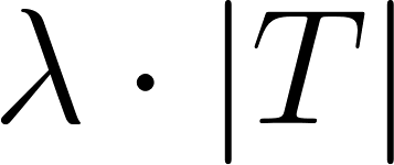 ) in examples 1 and 3, a hard depth cap everywhere, hoist mutation in examples 2, 3, and 4, and a length-capped rewrite in example 4.
- Fitness evaluation must stay computable and discriminative. Protected operators and finite returns (example 1), never-matching guards on exponentially slow regexes (example 3), and a grid resolution coarse enough to keep plants sparse (example 4) are all examples of the same engineering duty.
- GP optimizes fitness cases, and stops there. The evolved regex rejects a valid time; the evolved plant rule differs from the hidden one. More fitness cases, held-out validation, and behavior-level tests are the difference between “fits the data” and “knows the rule”.
The chapter-level takeaway is that GP is the right tool precisely when you want the structure and cannot write it down beforehand: formulas, controllers, parsers, schedules. When you only need coefficients inside a known model class, use ordinary fitting. GP is slower and its output needs curation (simplify, validate, guard), but its answers are readable programs.
For larger work, use DEAP or gplearn. Their GP modules implement this same loop (typed trees, guarded operators, tournament selection, parsimony or multi-objective size control), and you can port every experiment here by swapping gp_core calls for theirs.
Practice problems
- Give GP
exp. Addexp(protected:math.expwith the argument clamped to[-50, 50]) to example 1’s function set. Rerun and measure: does the evolved formula now express damping? Does its tree grow? What doesPARSIMONYneed to become to keep it small? - NAND-only synthesis. Rewrite example 2’s function set to
{NAND: 2}. The truth table is unchanged. NAND is functionally complete, so the optimum is reachable, but the search space is deeper. How many generations does the 32-row interlock now need? Then try parity-of-4 ( ) as the specification and observe why parity is the classic GP difficulty.
- A second regex, blindfolded. Point example 3 at a new task (US five-digit ZIP codes plus four-digit extensions, or
dd.mm.yyyydates): swapPOSITIVE/NEGATIVEand re-generalizeTERMINAL_FRAGMENTS. Keepprefix_creditand the quantifier guard; watch where the partial credit does and does not help, and design an example set that punishes the overfit you find. - Different angle, different plant. Set example 4’s
TURN_DEGto 60, 45, 90 and rerun. At 90 degrees plants degenerate into grid-aligned snakes; at 60 the target rule becomes easier. Report which angle gives the fastest convergence and explain the result in terms of cell collisions (the mechanism behind the “same phenotype, different genotype” observation). - Selection pressure dial. In example 4 replace tournament size 6 with 2, 10, and 30 (with
k=30you get near-greedy selection). Plot generations-to-0 against tournament size. Explain the shape of that curve with one sentence about diversity. - Initialization methods. Example 1 seeds its population with
method="half"; examples 2-4 use"grow". Rerun example 1 with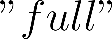 and with
 "grow"across five seeds each. Compare the generation-0 best MSE and the final size of the winner. Write the result in three sentences; the honest answer is “usually a little, and not reliably.” - Validation split. Modify example 3 to train on a random half of the positives and report fitness on the other half. The textbook regex should now beat the two-branch overfit. That single change is the difference between a demo and a system.
- Paper GP. Using the four-individual example in “One generation by hand”, run two more generations with tournament size 2, a crossover rate of 1.0, and no mutation, keeping one elite. Record the population after each generation and explain why the average fitness falls even though no new program was designed.
- Design a fitness function, then break it. Pick a task you know well: valid email addresses, a bowling score, a pizza order. Write down the primitive sets and a fitness function, then find a degenerate program that scores well without solving the task. Every loophole you find is a lesson about specifications.
- Watch the bloat. Run example 1 with
PARSIMONY = 0.0and print the winner’s size each generation. How large does it get in 40 generations? Restore the penalty and compare the final size and MSE. - Turn the pressure dial. Run example 1 with tournament sizes 2, 7, and 15 on the same
SEED. Record the generation at which the best MSE first drops below 0.10, and the final size. Explain the differences in one paragraph about diversity. - Your own problem. Choose a small task with a clear score: a text-formatting rule, a simple game strategy, a unit-conversion formula. Write down the terminals, the functions, and the fitness cases before you write any code, then reuse
gp_core.pyunchanged. Report what surprised you.
Glossary
ADF (automatically defined function). A subtree that evolution reuses by name, so repeated structure is encoded once. A step beyond plain tree GP.
Allele. The value stored at a gene. In tree GP, the symbol at a node: a function name or a terminal.
Bloat. Growth in program size that does not improve fitness. See “Bloat: why programs grow”.
Closure. The property that every function accepts every value the primitive set can produce. Protected operators restore closure.
Crossover (recombination). Building an offspring by exchanging parts of two parents; in tree GP, swapping two subtrees.
Elitism. Copying the best individuals into the next generation unchanged.
Ephemeral Random Constant (ERC). A new random constant drawn whenever a terminal leaf is created, so constants are re-invented every generation and tuned by selection.
Fitness. The scalar score used by selection. This chapter minimizes it.
Fitness case. One test input, with its expected output.
Function set. The internal nodes available to a program, each with a fixed arity.
Generation. One cycle of selection and reproduction.
Genotype. The representation that is copied and varied (here, the tree). Compare phenotype.
Hoist mutation. Replacing a node with one of its own descendants, which can only shrink the program.
Individual. One candidate program.
Initialization. How the first generation is built: full, grow, half-and-half, or ramped half-and-half.
Mutation. A random change to one individual.
Parsimony pressure. A fitness penalty proportional to program size, used to control bloat.
Phenotype. The behavior a genotype produces: the formula, circuit, regex, or plant.
Population. The set of individuals alive at one time.
Premature convergence. Losing diversity and settling on a mediocre answer before the search has explored enough.
Protected operator. A function that returns a safe value instead of raising, such as division that returns 1.0 for a near-zero denominator.
Selection pressure. How strongly selection favors the best individuals. Tournament size is the usual dial.
Subtree. A node together with all of its descendants; the unit of crossover and mutation.
Sufficiency. The property that the primitive set can express a solution at all.
Terminal set. The leaves available to a program: variables, constants, and generated constants.
Tournament selection. Drawing k individuals at random and keeping the best.
Tree depth and size. Depth is the longest root-to-leaf path, counted in nodes; size is the total node count.
Further reading
- John R. Koza, Genetic Programming: On the Programming of Computers by Means of Natural Selection, MIT Press, 1992. The book that defined the field and the source of full/grow initialization and the standard benchmark problems.
- Wolfgang Banzhaf, Peter Nordin, Robert E. Keller and Frank D. Francone, Genetic Programming: An Introduction, Morgan Kaufmann, 1998. A textbook that covers the representation and the main variants.
- William B. Langdon and Riccardo Poli, Foundations of Genetic Programming, Springer, 2002. The theory: schemata, bloat, and convergence.
- Riccardo Poli, William B. Langdon and Nicholas F. McPhee, A Field Guide to Genetic Programming, 2008, free online at https://www.gp-field-guide.org.uk/. The best single next read after this chapter.
- The genetic programming bibliography, https://gpbib.pmacs.upenn.edu/, maintains the literature going back to the 1950s.
- Michael Schmidt and Hod Lipson, “Distilling free-form natural laws from experimental data”, Science, 2009. A landmark symbolic regression result that rediscovered physical laws from measurements.
- For production work, use DEAP (https://deap.readthedocs.io) or gplearn (https://gplearn.readthedocs.io). Both implement this chapter’s loop with typed trees, guarded operators, and multi-objective size control, so you can port any experiment by swapping
gp_corecalls for theirs.