“Classic” Machine Learning
“Classic” Machine Learning (ML) is a broad field that encompasses a variety of algorithms and techniques for learning from data. These techniques are used to make predictions, classify data, and uncover patterns and insights. Some of the most common types of classic ML algorithms include:
- Linear regression: a method for modeling the relationship between a dependent variable and one or more independent variables by fitting a linear equation to the observed data.
- Logistic regression: a method for modeling the relationship between a binary dependent variable and one or more independent variables by fitting a logistic function to the observed data.
- Decision Trees: a method for modeling decision rules based on the values of the input variables, which are organized in a tree-like structure.
- Random Forest: a method that creates multiple decision trees and averages the results to improve the overall performance of the model
- K-Nearest Neighbors (K-NN): a method for classifying data by finding the K-nearest examples in the training data and assigning the most similar common class among them.
- Naive Bayes: a method for classifying data based on Bayes’ theorem and the assumption of independence between the input variables.
We will be covering a very small subset of “classic” ML, and then dive deeper into Deep Learning in later chapters. Deep Learning differs from classic ML in several ways:
- Scale: Classic ML algorithms are typically designed to work with small to medium-sized datasets, while deep learning algorithms are designed to work with large-scale datasets, such as millions or billions of examples.
- Architecture: Classic ML algorithms have a relatively shallow architecture, with a small number of layers and parameters, while deep learning algorithms have a deep architecture, with many layers and millions or billions of parameters.
- Non-linearity: Classic ML algorithms are sometimes linear, (i.e., the relationship between the input and output is modeled by a linear equation), while deep learning algorithms are non-linear, (i.e., the relationship is modeled by a non-linear function).
- Feature extraction: “Classic” ML requires feature extraction, which is the process of transforming the raw input data into a set of features that can be used by the algorithm. Deep learning can automatically learn features from raw data, so it does not usually require too much separate effort for feature extraction.
So, Deep Learning is a subfield of machine learning that is focused on the design and implementation of artificial neural networks with many layers which are capable of learning from large-scale and complex data. It is characterized by its deep architecture, non-linearity, and ability to learn features from raw data, which sets it apart from “classic” machine learning algorithms.
Example Material
Here we cover just a single example of what I think of as “classic machine learning” using the scikit-learn Python library. Later we cover deep learning in three separate chapters. Deep learning models are more general and powerful but it is important to recognize the types of problems that can be solved using the simpler techniques.
The only requirements for this chapter are:
1 uv pip install scikit-learn pandas
Please note that the content in this book is heavily influenced by what I use in my own work. I mostly use deep learning so its coverage comprises half this book. For this classic machine learning chapter I only use a classification model. I will not be covering regression or clustering models.
We will use the same Wisconsin cancer dataset for both the following classification example and a deep learning classification example in a later chapter. Here are the first few rows of the file labeled_cancer_data.csv:
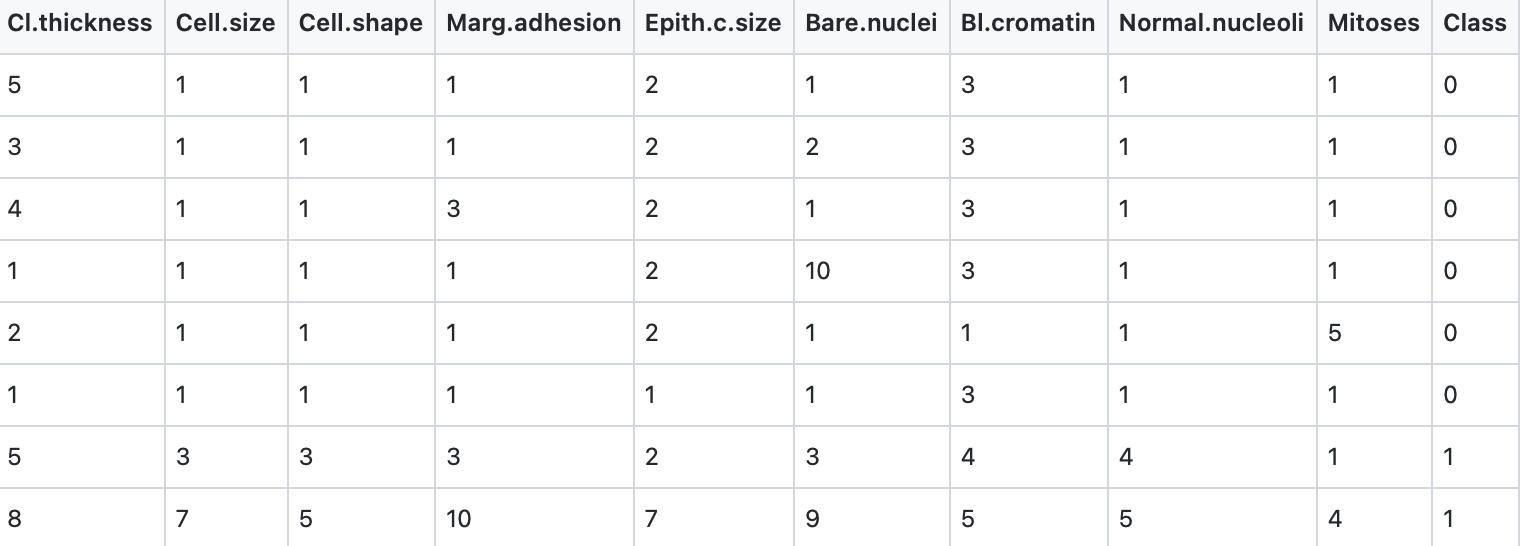
The last column class indicates the class of the sample, 0 for non-malignant and 1 for malignant. The scikit-learn library has high level and simple to use utilities for reading CSV (spreadsheet) data and for preparing the data for training and testing. I don’t use these utilities here because I am reusing the data loading code from the later deep learning example.
We will use the Pandas library and if you have not used Pandas before you might want to reference the Pandas documentation. Here is a summary of why Pandas is generally useful: it is a popular Python library for data manipulation and analysis that provides data structures and data analysis tools for working with structured data (often spreadsheet data). One of the key data structures in Pandas is the DataFrame, which is a two-dimensional table of data with rows and columns.
A DataFrame is essentially a labeled, two-dimensional array, where each column has a name and each row has an index. DataFrames are similar to tables in a relational database or data in a spreadsheet. They can be created from a variety of data sources such as CSV, Excel, SQL databases, or even Python lists and dictionaries. They can also be transformed, cleaned, and manipulated using a wide range of built-in methods and functionalities.
Pandas DataFrames provide a lot of functionalities to handle and process data. The most common ones are:
- Indexing: data can be selected by its label or index.
- Filtering: data can be filtered by any condition.
- Grouping: data can be grouped by any column.
- Merging and joining: data can be joined or merged with other data.
- Data type conversion: data can be converted to any data type.
- Handling missing data: data can be filled in or removed based on any condition.
DataFrames are widely used in data science and machine learning projects for loading, cleaning, processing, and analyzing data. They are also used for data visualization, data preprocessing, and feature engineering tasks.
Listing of load_data.py:
 1 import pandas as pd
 2
 3
 4 def load_data():
 5     train_df = pd.read_csv("labeled_cancer_data.csv")
 6     test_df = pd.read_csv("labeled_test_data.csv")
 7
 8     train = train_df.to_numpy()
 9     X_train = train[:, 0:9].astype(float)  # 9 input features
10     print("Number training examples:", len(X_train))
11     # Training target: one output (0 for non-malignant, 1 for malignant)
12     Y_train = train[:, -1].astype(float)
13
14     test = test_df.to_numpy()
15     X_test = test[:, 0:9].astype(float)
16     Y_test = test[:, -1].astype(float)
17     print("Number testing examples:", len(X_test))
18     return (X_train, Y_train, X_test, Y_test)
In line 6 we read the CSV training data into a Pandas DataFrame. In line 9 we convert the DataFrame to a NumPy array using the to_numpy() method (preferred over the older .values property). In line 10 we copy all rows of data, skipping the last column (target classification we want to be able to predict) and converting all data to floating point numbers. In line 13 we copy just the last column of the training data array for use as the target classification.
Classification Models using Scikit-learn
Classification is a type of supervised machine learning problem where the goal is to predict the class or category of an input sample based on a set of features. The goal of a classification model is to learn a mapping from the input features to the output class labels.
Scikit-learn (sklearn) is a popular Python library for machine learning that is effective for several reasons (partially derived from the Skikit-learn documentation):
- Scikit-learn provides a consistent and intuitive API for a wide range of machine learning models, which makes it easy to switch between different algorithms and experiment with different approaches.
- Scikit-learn includes a large collection of models for supervised, unsupervised, and semi-supervised learning (e.g., linear and non-linear models, clustering, and dimensionality reduction).
- Scikit-learn includes a wide range of preprocessing and data transformation tools, such as feature scaling, one-hot encoding, feature extraction, and more, that can be used to prepare and transform the data before training the model.
- Scikit-learn provides a variety of evaluation metrics, such as accuracy, precision, recall, F1-score, and more, that can be used to evaluate the performance of a model on a given dataset.
- Scikit-learn is designed to be scalable, which means it can handle large datasets and high-dimensional feature spaces. It also provides tools for parallel and distributed computing, which can be used to speed up the training process on large datasets.
- Scikit-learn is designed to be easy to use, with clear and concise code, a well-documented API, and plenty of examples and tutorials that help users get started quickly.
- Scikit-learn is actively developed and maintained, with regular updates and bug fixes, and a large and active community of users and developers who contribute to the library and provide support through mailing lists, forums, and other channels.
All these features make Scikit-learn a powerful and widely used machine learning library for various types of machine learning tasks.
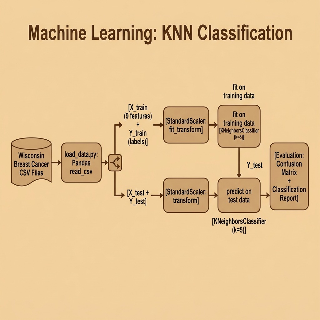
 1 from sklearn.preprocessing import StandardScaler
 2 from sklearn.neighbors import KNeighborsClassifier
 3 from sklearn.metrics import classification_report, confusion_matrix
 4
 5 from load_data import load_data
 6
 7 (X_train, Y_train, X_test, Y_test) = load_data()
 8
 9 # Remove mean and scale to unit variance:
10 scaler = StandardScaler()
11 X_train = scaler.fit_transform(X_train)
12 X_test = scaler.transform(X_test)
13
14 # Use the KNN classifier to fit data:
15 classifier = KNeighborsClassifier(n_neighbors=5)
16 classifier.fit(X_train, Y_train)
17
18 # Predict y data with classifier:
19 y_predict = classifier.predict(X_test)
20
21 # Print results:
22 print(confusion_matrix(Y_test, y_predict))
23 print(classification_report(Y_test, y_predict))
Note that we fit the StandardScaler on the training data and then use the same fitted scaler to transform the test data. This is important: scaling the test data with parameters learned from the training set prevents data leakage and ensures a fair evaluation.
We can now train and test the model and evaluate how accurate the model is. In reading the following output, you should understand a few definitions. In machine learning, precision, recall, F1-score, and support are all metrics used to evaluate the performance of a classification model, specifically in regards to binary classification:
- Precision: the proportion of true positive predictions out of the total of all positive predictions made by the model. It is a measure of how many of the positive predictions were actually correct.
- Recall: the proportion of true positive predictions out of all actual positive observations in the data. It is a measure of how well the model is able to find all the positive observations.
- F1-score: the harmonic mean of precision and recall. It is a measure of the balance between precision and recall and is generally used when you want to seek a balance between precision and recall.
- Support: number of observations in each class.
These metrics provide an overall view of a model’s performance in terms of both correctly identifying positive observations and avoiding false positive predictions.
 1 $ python classification.py
 2 Number training examples: 554
 3 Number testing examples: 15
 4 [[8 1]
 5  [0 6]]
 6               precision    recall  f1-score   support
 7
 8          0.0       1.00      0.89      0.94         9
 9          1.0       0.86      1.00      0.92         6
10
11     accuracy                           0.93        15
12    macro avg       0.93      0.94      0.93        15
13 weighted avg       0.94      0.93      0.93        15
Classic Machine Learning Wrap-up
I have already admitted my personal biases in favor of deep learning over simpler machine learning and I proved that by using perhaps only 1% of the functionality of Scikit-learn in this chapter.
Optional Practice Problems
To help solidify your understanding of “classic” machine learning with scikit-learn, try implementing the following practice problems by extending the existing code examples.
1. Easy: Hyperparameter Tuning for K-NN
Objective: Understand how the choice of  (number of neighbors) affects model performance.
Task:
- Open classification.py.
- Modify the script to loop over different values of
n_neighbors(for example, odd numbers from 1 to 15:[1, 3, 5, 7, 9, 11, 13, 15]). -
For each value of:
- Initialize and fit the
KNeighborsClassifier. - Calculate and print the classification accuracy on the test set.
- Identify which value of provides the best performance and explain why choosing an even vs. odd value for matters in binary classification.
2. Medium: Comparing Classifiers
Objective: Compare the K-Nearest Neighbors classifier against other classic machine learning algorithms covered in this chapter.
Task:
- Create a new script in /Users/markwatson/GITHUB/PythonAIBook/source-code/machine-learning/ (e.g.,
compare_classifiers.py) that loads the data using load_data.py. -
Import at least two other classifiers from scikit-learn, such as:
- Logistic Regression (
sklearn.linear_model.LogisticRegression) - Decision Tree (
sklearn.tree.DecisionTreeClassifier) - Random Forest (
sklearn.ensemble.RandomForestClassifier)
- Train each classifier on the scaled training data and evaluate them on the test dataset.
- Print the confusion matrix and classification report for each.
- Write a brief summary comparing the precision, recall, and F1-score of the alternative classifiers with the K-NN baseline.
3. Hard: Implementing Cross-Validation
Objective: Use cross-validation to get a more robust estimate of model performance, rather than relying on a single, fixed train/test split.
Task:
- Create a script (e.g.,
cross_validation.py) that reads both labeled_cancer_data.csv and labeled_test_data.csv using Pandas. - Concatenate these two datasets into a single dataset.
- Separate the features and target labels from the combined dataset.
- Use
sklearn.model_selection.cross_val_scoreorsklearn.model_selection.KFoldto perform 5-fold cross-validation using theKNeighborsClassifier. - Apply feature scaling correctly within each fold using a pipeline (
sklearn.pipeline.Pipeline) containingStandardScalerandKNeighborsClassifierto avoid data leakage. - Calculate and print the mean and standard deviation of the accuracy across all 5 folds.