Overview of Reinforcement Learning (Optional Material)
Reinforcement Learning has been used in various applications such as robotics, game playing, recommendation systems, and more. Reinforcement Learning (RL) is a broad topic and we will only cover basic aspects of RL.
The requirements for this chapter are:
1 uv pip install gymnasium numpy pymdptoolbox
The examples for this chapter are in the directory source-code/reinforcement_learning.
Overview
Reinforcement Learning is a type of machine learning that is concerned with decision-making in dynamic and uncertain environments. RL uses the concept of an agent which interacts with its environment by taking actions and receiving feedback in the form of rewards or penalties. The goal of the agent is to learn a policy which is a mapping from states of the environment to actions with the goal of maximizing the expected cumulative reward over time.
There are several key components to RL:
- Environment: the system or “world” that the agent interacts with.
- Agent: the decision-maker that chooses actions based on its current state, the current environment, and its policy.
- State: a representation of the current environment, the parameters and trained policy of the agent, and possibly the visible actions of other agents in the environment.
- Action: a decision taken by the agent.
- Reward: a scalar value that the agent receives as feedback for its actions.
Reinforcement learning algorithms can be divided into two main categories: value-based and policy-based. In value-based RL the agent learns an estimate of the value of different states or state-action pairs which are then used to determine the optimal policy. In contrast, in policy-based RL the agent directly learns a policy without estimating the value of states or state-action pairs.
Reinforcement Learning can be implemented using different techniques such as Q-learning, SARSA, DDPG, A2C, PPO, etc. Some of these techniques are model-based, which means that the agent uses a model of the environment to simulate the effects of different actions and plan ahead. Others are model-free, which means that the agent learns directly from the rewards and transitions experienced in the environment.
If you enjoy the overview material in this chapter I recommend that you consider investing the time in the Coursera RL specialization https://www.coursera.org/learn/fundamentals-of-reinforcement-learning taught by Martha and Adam White. There are 50+ RL courses on Coursera. I took the courses taught by Martha and Adam White before starting my RL project at Capital One.
My favorite RL book is “Reinforcement Learning: An Introduction, second edition” by Richard Sutton and Andrew Barto, that can be read online for free at http://www.incompleteideas.net/book/the-book-2nd.html. They originally wrote their book examples in Common Lisp but most of the code is available rewritten in Python. The Common Lisp code for the examples is here. Shangtong Zhang translated the book examples to Python, available here. Martha and Adam White’s Coursera class uses this book as a reference.
The core idea of RL is that we train a software agent to interact with and change its environment based on its expectations of the utility of current actions improving metrics for success in the future. There is some tension between writing agents that simply reuse past actions that proved to be useful, rather than aggressively exploring new actions in the environment. There are interesting formalisms for this that we will cover.
There are two general approaches to providing training environments to Reinforcement Learning trained agents: physically devices in the real world or simulated environments. This is not a book on robotics so we use the second option.
The end goal for modeling a RL problem is calculating a policy that can be used to control an agent in environments that are similar to the training environment. In a model at time t we have a given Statet. RL policies can be continually be updated during training and in production environments. A policy given a Statet, calculates an Actiont to execute and changes the state to Statet+1.
Available RL Tools
For initial experiments with RL, I would recommend taking the same path that I took before using RL at work:
- Using a maintained fork of OpenAI’s Gym library Gymnasium.
- Taking the Coursera classes by Martha and Adam White.
- The Sutton/Barto RL Book and accompanying Common Lisp or Python examples.
The original OpenAI RL Gym was a good environment for getting started with simple environments and examples but I didn’t get very far with self-study. The RL Coursera classes were a great overview of theory and practice, and I then spend as much time as I could spare working through Sutton/Barto before my project started.
An Introduction to Markov Decision Process
Before we can write a reinforcement learning agent, we need to understand the mathematical framework that RL is built upon: the Markov Decision Process (MDP). An MDP provides a formal way to model sequential decision-making problems where outcomes are partly random and partly under the control of a decision-maker.
Let’s start by defining the key terms:
Sequential decision problem: a problem where decisions are made in sequence over time, and each decision affects future states and rewards. Unlike one-shot classification or regression, you must think ahead.
Fully observable: the agent can see the complete state of the environment at each step. No hidden information or partial views.
Stochastic environment: transitions between states are not deterministic. An action taken in a given state may lead to different outcomes with certain probabilities. The real world is uncertain, and MDPs model this uncertainty.
Markov property: the future depends only on the current state and action, not on the history of how you got there. Formally, P(Statet+1 | Statet, Actiont) = P(Statet+1 | Statet, Actiont, Statet-1, Actiont-1, …).
Bellman equation: the recursive relationship that expresses the value of a state as the expected immediate reward plus the discounted value of the next state. This is the foundation of dynamic programming in RL: V(s) = max_a [ R(s,a) + γ Σ P(s’|s,a) V(s’) ] where γ (gamma) is the discount factor.
The discount factor γ (between 0 and 1) controls how much the agent values future rewards versus immediate rewards:
- γ close to 0: agent is shortsighted, cares mostly about immediate reward
- γ close to 1: agent is farsighted, cares about long-term cumulative reward
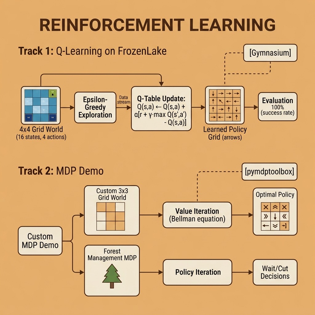
Solving MDPs with pymdptoolbox
The pymdptoolbox library provides classic MDP solution algorithms. Let’s work through two examples: a custom grid world and the built-in forest management problem.
Listing of mdp_demo.py:
 1 import mdptoolbox.example
 2 import numpy as np
 3
 4 print("=" * 55)
 5 print("Markov Decision Process Demo")
 6 print("=" * 55)
 7
 8 print("\n--- Example 1: Custom 3x3 Grid World ---")
 9 n_states = 9
10 n_actions = 4
11
12 P = np.zeros((n_actions, n_states, n_states))
13 grid = [(r, c) for r in range(3) for c in range(3)]
14 for s, (r, c) in enumerate(grid):
15     for a, (dr, dc) in enumerate([(-1, 0), (0, 1), (1, 0), (0, -1)]):
16         nr, nc = r + dr, c + dc
17         if 0 <= nr < 3 and 0 <= nc < 3:
18             ns = nr * 3 + nc
19         else:
20             ns = s
21         P[a, s, ns] = 1.0
22
23 R = np.zeros((n_states, n_actions))
24 R[8, :] = 10.0
25 R[5, :] = -5.0
26
27 vi = mdptoolbox.mdp.ValueIteration(P, R, 0.9)
28 vi.run()
29 actions = ["↑", "→", "↓", "←"]
30 print("Optimal policy:")
31 for r in range(3):
32     row = ""
33     for c in range(3):
34         s = r * 3 + c
35         row += f"  {actions[vi.policy[s]]}  "
36     print(row)
37 print(f"\nValue function: {np.round(vi.V, 2)}")
38 print(f"Iterations to converge: {vi.iter}")
39
40 print("\n--- Policy Iteration on same grid ---")
41 pi = mdptoolbox.mdp.PolicyIteration(P, R, 0.9)
42 pi.run()
43 print(f"Policy: {tuple(pi.policy)}")
44 print(f"Iterations: {pi.iter}")
45
46 print("\n--- Example 2: Forest Management (built-in) ---")
47 P2, R2 = mdptoolbox.example.forest(S=5, r1=4, r2=2, p=0.1)
48 print("States: 5 (forest age classes 0-4)")
49 print("Action 0 = Wait, Action 1 = Cut")
50 print("p(fire) = 0.1 each year")
51 print(f"Reward shape: {R2.shape} (states × actions)")
52
53 vi2 = mdptoolbox.mdp.ValueIteration(P2, R2, 0.9)
54 vi2.run()
55 print(f"Optimal policy: {tuple(vi2.policy)}")
56 for s, a in enumerate(vi2.policy):
57     print(f"  Forest age {s}: {'Wait' if a == 0 else 'Cut'}")
58 print(f"Value function: {np.round(vi2.V, 2)}")
59 print(f"Iterations: {vi2.iter}")
Here is the output of running mdp_demo.py (the unicode characters for directionsin the Optimal policy output don’t print correctly):
 1 $ python mdp_demo.py
 2 =======================================================
 3 Markov Decision Process Demo
 4 =======================================================
 5
 6 --- Example 1: Custom 3x3 Grid World ---
 7 Optimal policy:
 8   →    ↓    ↓
 9   →    ↓    ↓
10   →    →    →
11
12 Value function: [ 6.56 13.85 17.45 13.85 21.95 25.95 21.95 30.95 40.95]
13 Iterations to converge: 5
14
15 --- Policy Iteration on same grid ---
16 Policy: (1, 2, 2, 1, 2, 2, 1, 1, 1)
17 Iterations: 5
18
19 --- Example 2: Forest Management (built-in) ---
20 States: 5 (forest age classes 0-4)
21 Action 0 = Wait, Action 1 = Cut
22 p(fire) = 0.1 each year
23 Reward shape: (5, 2) (states × actions)
24 Optimal policy: (0, 0, 0, 0, 0)
25   Forest age 0: Wait
26   Forest age 1: Wait
27   Forest age 2: Wait
28   Forest age 3: Wait
29   Forest age 4: Wait
30 Value function: [ 3.49  5.62  8.24 11.48 15.48]
31 Iterations: 6
Walking through Example 1, we create a 3×3 grid where each cell is a state (0 through 8). The agent can move up, right, down, or left. The transition matrix P has shape (actions, states, states) — for each action and current state, it specifies the probability of landing in each next state. Our grid is deterministic (probability of 1.0 for each move), and bumping into walls keeps the agent in place.
The reward matrix R gives 10 for reaching the goal (bottom-right, state 8) and -5 for the trap (state 5, which is the middle-right cell). Value iteration converges in 5 iterations and produces a sensible policy: the arrows point around the trap toward the goal. The value function shows that states closer to the goal have higher values.
I also ran Policy Iteration on the same grid. Both algorithms arrived at the same policy but through different means: value iteration improves value estimates until convergence, while policy iteration alternates between evaluating a fixed policy and improving it greedily.
In Example 2, we use pymdptoolbox’s built-in forest management problem. At each year, you choose to Wait (let the forest grow one age class) or Cut (harvest timber, resetting the forest to age 0). There is a 10% chance of fire each year that also resets the forest to age 0. With these parameters the optimal policy is to always Wait — the expected value of older forest outweighs the immediate reward of cutting.
The key takeaway: MDPs give you a formal language to describe decision problems, and algorithms like value iteration and policy iteration compute optimal policies. In the next section, we will tackle environments where we do not know the transition probabilities in advance — which is where reinforcement learning comes in.
A Concrete Example: Q-Learning with Gymnasium
When the transition and reward models are unknown, the agent must learn through trial and error. Q-learning is one of the simplest and most widely used model-free RL algorithms. It learns an action-value function Q(s,a) — the expected cumulative reward of taking action a in state s and following the optimal policy thereafter.
The Q-learning update rule is:
Q(s,a) ← Q(s,a) + α [ r + γ · max_a’ Q(s’,a’) — Q(s,a) ]
Where:
- α (alpha) is the learning rate
- γ (gamma) is the discount factor
- r is the immediate reward received
- s’ is the next state
The agent also needs to balance exploration (trying random actions to discover better strategies) against exploitation (using known good actions). We use an epsilon-greedy strategy: with probability ε, take a random action; otherwise take the action with the highest Q-value. Over time we decay ε so the agent explores less and exploits more.
We will use Gymnasium (the maintained successor to OpenAI Gym) and its FrozenLake environment. In FrozenLake, the agent navigates a 4×4 grid of frozen and cracked ice to reach a goal without falling through. By default, the ice is slippery — your intended move only succeeds with 1/3 probability, and you slide perpendicular otherwise.
Listing of frozen_lake_qlearning.py:
  1 import gymnasium as gym
  2 import numpy as np
  3
  4 np.random.seed(42)
  5
  6
  7 def q_learning(env, episodes=10000, alpha=0.1, gamma=0.99,
  8                epsilon=1.0, epsilon_decay=0.999, min_epsilon=0.01):
  9     n_states = env.observation_space.n
 10     n_actions = env.action_space.n
 11     Q = np.zeros((n_states, n_actions))
 12     success_history = []
 13
 14     for episode in range(episodes):
 15         state, _ = env.reset()
 16         done = False
 17
 18         while not done:
 19             if np.random.random() < epsilon:
 20                 action = env.action_space.sample()
 21             else:
 22                 action = np.argmax(Q[state])
 23
 24             next_state, reward, terminated, truncated, _ = env.step(action)
 25             done = terminated or truncated
 26
 27             best_next = np.max(Q[next_state])
 28             Q[state, action] += alpha * (
 29                 reward + gamma * best_next - Q[state, action]
 30             )
 31
 32             state = next_state
 33
 34         epsilon = max(min_epsilon, epsilon * epsilon_decay)
 35
 36         if (episode + 1) % 1000 == 0:
 37             success_rate = evaluate(env, Q, episodes=100)
 38             success_history.append((episode + 1, success_rate))
 39             print(f"  Episode {episode + 1:>5}: success rate = {success_rate:.2f}")
 40
 41     return Q, success_history
 42
 43
 44 def evaluate(env, Q, episodes=100):
 45     successes = 0
 46     for _ in range(episodes):
 47         state, _ = env.reset()
 48         done = False
 49         while not done:
 50             action = np.argmax(Q[state])
 51             state, reward, terminated, truncated, _ = env.step(action)
 52             done = terminated or truncated
 53             if terminated and reward == 1.0:
 54                 successes += 1
 55     return successes / episodes
 56
 57
 58 def print_policy(Q, env_name):
 59     n_states = Q.shape[0]
 60     size = int(np.sqrt(n_states))
 61     arrows = {0: "←", 1: "↓", 2: "→", 3: "↑"}
 62
 63     print(f"\nLearned policy for {env_name}:")
 64     for row in range(size):
 65         row_str = ""
 66         for col in range(size):
 67             s = row * size + col
 68             row_str += arrows[np.argmax(Q[s])]
 69         print(f"  {row_str}")
 70     print("  (←=left ↓=down →=right ↑=up)")
 71
 72
 73 print("=" * 55)
 74 print("Q-Learning on FrozenLake (slippery)")
 75 print("=" * 55)
 76
 77 env = gym.make("FrozenLake-v1", is_slippery=True)
 78 print(f"States: {env.observation_space.n}")
 79 print(f"Actions: {env.action_space.n}")
 80 print(f"Map size: 4x4")
 81
 82 print("\nTraining:")
 83 Q, history = q_learning(env)
 84
 85 print_policy(Q, "FrozenLake-v1 (slippery)")
 86
 87 print("\nFinal evaluation (1000 episodes):")
 88 final_rate = evaluate(env, Q, episodes=1000)
 89 print(f"  Success rate: {final_rate:.2f}")
 90
 91 print("\n" + "=" * 55)
 92 print("Q-Learning on FrozenLake (deterministic, no slipping)")
 93 print("=" * 55)
 94
 95 env2 = gym.make("FrozenLake-v1", is_slippery=False)
 96 print(f"States: {env2.observation_space.n}")
 97 print(f"Actions: {env2.action_space.n}")
 98
 99 print("\nTraining:")
100 Q2, _ = q_learning(env2, episodes=2000)
101
102 print_policy(Q2, "FrozenLake-v1 (deterministic)")
103
104 print("\nFinal evaluation (1000 episodes):")
105 final_rate2 = evaluate(env2, Q2, episodes=1000)
106 print(f"  Success rate: {final_rate2:.2f}")
107
108 env.close()
109 env2.close()
Here is the output:
 1 $ python frozen_lake_qlearning.py
 2 =======================================================
 3 Q-Learning on FrozenLake (slippery)
 4 =======================================================
 5 States: 16
 6 Actions: 4
 7 Map size: 4x4
 8
 9 Training:
10   Episode  1000: success rate = 0.68
11   Episode  2000: success rate = 0.77
12   Episode  3000: success rate = 0.69
13   Episode  4000: success rate = 0.75
14   Episode  5000: success rate = 0.77
15   Episode  6000: success rate = 0.50
16   Episode  7000: success rate = 0.77
17   Episode  8000: success rate = 0.77
18   Episode  9000: success rate = 0.70
19   Episode 10000: success rate = 0.75
20
21 Learned policy for FrozenLake-v1 (slippery):
22   ←↑↑↑
23   ←←→←
24   ↑↓←←
25   ←→↓←
26   (←=left ↓=down →=right ↑=up)
27
28 Final evaluation (1000 episodes):
29   Success rate: 0.74
30
31 =======================================================
32 Q-Learning on FrozenLake (deterministic, no slipping)
33 =======================================================
34 States: 16
35 Actions: 4
36
37 Training:
38   Episode  1000: success rate = 1.00
39   Episode  2000: success rate = 1.00
40
41 Learned policy for FrozenLake-v1 (deterministic):
42   ↓←←←
43   ↓←↓←
44   →→↓←
45   ←→→←
46   (←=left ↓=down →=right ↑=up)
47
48 Final evaluation (1000 episodes):
49   Success rate: 1.00
The q_learning function implements the core algorithm. We maintain a Q-table of shape (n_states, n_actions) initialized to zeros. Each episode runs until termination (falling in a hole or reaching the goal) or truncation (100-step limit). The epsilon-greedy strategy decays from 1.0 (pure exploration) to 0.01 over time, following the decay schedule epsilon *= 0.999 each episode.
The Q-value update is the heart of Q-learning:
1 best_next = np.max(Q[next_state])
2 Q[state, action] += alpha * (reward + gamma * best_next - Q[state, action])
This says: move Q(s,a) a small step (controlled by alpha) toward r + γ·max_a' Q(s',a'). The difference r + γ·max Q - Q is called the temporal-difference error — how much better or worse the outcome was than predicted.
Let’s discuss the results:
Slippery version: Achieves ~75% success rate after 10,000 episodes. This is about as good as tabular Q-learning gets on the slippery FrozenLake — the randomness of ice physics means some runs are doomed regardless of policy. The learned policy arrows point toward the goal, though the randomness makes the policy harder to interpret visually than the deterministic case. You can also see the success rate fluctuate (e.g., dropping to 0.50 at episode 6000) — this is normal for Q-learning on stochastic environments and reflects the exploration-exploitation trade-off.
Deterministic version (is_slippery=False): Converges to a 100% success rate within 1,000 episodes. Without slipping, the task reduces to a simple shortest-path problem and Q-learning finds it quickly.
Other Gymnasium Environments Worth Exploring
Once you are comfortable with FrozenLake, Gymnasium offers many environments to experiment with:
- Taxi-v3: 500 discrete states, the agent must pick up and drop off a passenger at correct locations. 5 actions (move directions + pickup/dropoff). Good for testing discrete Q-learning at slightly larger scale.
- CartPole-v1: balance a pole on a cart. Continuous observation space (4 values), discrete actions (2). Requires function approximation (e.g., a neural network) rather than a Q-table.
- MountainCar-v0: drive an underpowered car up a hill. Continuous observations, discrete actions. Classic example where exploration strategy matters deeply.
- LunarLander-v3: land a spacecraft on a landing pad. 8 continuous observations, 4 discrete actions. More complex dynamics.
For continuous observation spaces, you cannot use a lookup table — you need Deep Q-Networks (DQN) which use neural networks to approximate Q(s,a). That topic is beyond our scope here, but the Sutton/Barto book covers it well.
When learning RL, start with tabular methods (Q-learning on discrete environments) before moving to deep RL. The concepts transfer directly, but debugging is far easier when you can inspect every Q-value in a table.
Reinforcement Learning Wrap-up
In this chapter we covered:
- Markov Decision Processes: the mathematical foundation of RL, including states, actions, rewards, transition probabilities, the Bellman equation, and discount factors.
- MDP solving with pymdptoolbox: value iteration and policy iteration on custom and built-in problems.
- Q-learning: a model-free algorithm that learns from experience without needing transition probabilities. We implemented it from scratch and trained agents on the FrozenLake environment.
- Exploration vs exploitation: controlled by the epsilon-greedy strategy with decaying epsilon.
If this chapter sparked your interest, I encourage you to work through the Coursera specialization by Martha and Adam White and the Sutton/Barto book. For Python-focused RL, the Stable-Baselines3 library provides reliable implementations of DQN, A2C, PPO, and other algorithms ready to use with Gymnasium environments.
I tagged this chapter as optional material because I believe most readers will get more immediate value from mastering deep learning and pre-trained models. But if you find yourself working on sequential decision-making problems — robotics, game AI, resource allocation, dynamic pricing — the RL toolkit becomes indispensable.
Optional Practice Problems
Problem 1: Parameter Sensitivity in Forest Management (Easy)
In the Forest Management example in mdp_demo.py, the optimal policy with a discount factor of  and a fire probability of
  is to always Wait.
- Modify the script to perform a parameter sweep over different discount factors
 and fire probabilities
  .
.
- Record the resulting optimal policy for each combination.
- Explain intuitively how a low discount factor (valuing short-term gains) or a high risk of fire (destroying progress) changes the agent’s behavior from “Wait” to “Cut”.
Problem 2: Implementing a Stochastic Grid World (Medium)
The 3x3 grid world in mdp_demo.py is completely deterministic: when the agent takes an action, it transitions to the target cell with a probability of 1.0.
- Modify the transition matrix creation in mdp_demo.py to model a slippery grid. If the agent chooses a movement action (e.g., move Right), it should succeed with a probability of 0.8. With a probability of 0.1, it slips to the left (perpendicularly), and with a probability of 0.1, it slips to the right. (Note: Bumping into a wall still results in staying in the same cell).
- Run both Value Iteration and Policy Iteration on this stochastic environment.
- Compare the resulting value function and optimal policy with the deterministic version. How does transition noise affect the expected cumulative rewards of the non-goal states?
Problem 3: Scaling Q-Learning to the 8x8 Frozen Lake (Hard)
The tabular Q-learning code in frozen_lake_qlearning.py is configured for the 4x4 FrozenLake-v1 map.
- Modify the script to use the larger 8x8 grid:
gym.make("FrozenLake-v1", map_name="8x8", is_slippery=True). - Train the agent using the original parameters. You will likely observe that the success rate remains extremely low (often close to 0) because the reward is sparse (only 1.0 at the goal) and the state space is four times larger.
-
Implement one or both of the following enhancements to solve the 8x8 grid:
- Hyperparameter Sweep: Write a search script to find optimal values for the learning rate
 , the decay rate of
  , and the number of training episodes (hint: you may need 50,000+ episodes).
- Reward Shaping: Implement a custom wrapper or modify the step loop to provide intermediate feedback. For example, give a small positive reward proportional to the decrease in Manhattan distance to the goal, or apply a step penalty (e.g., -0.01) for non-goal steps to discourage circular paths.
- Report your final success rate and compare it against the baseline.