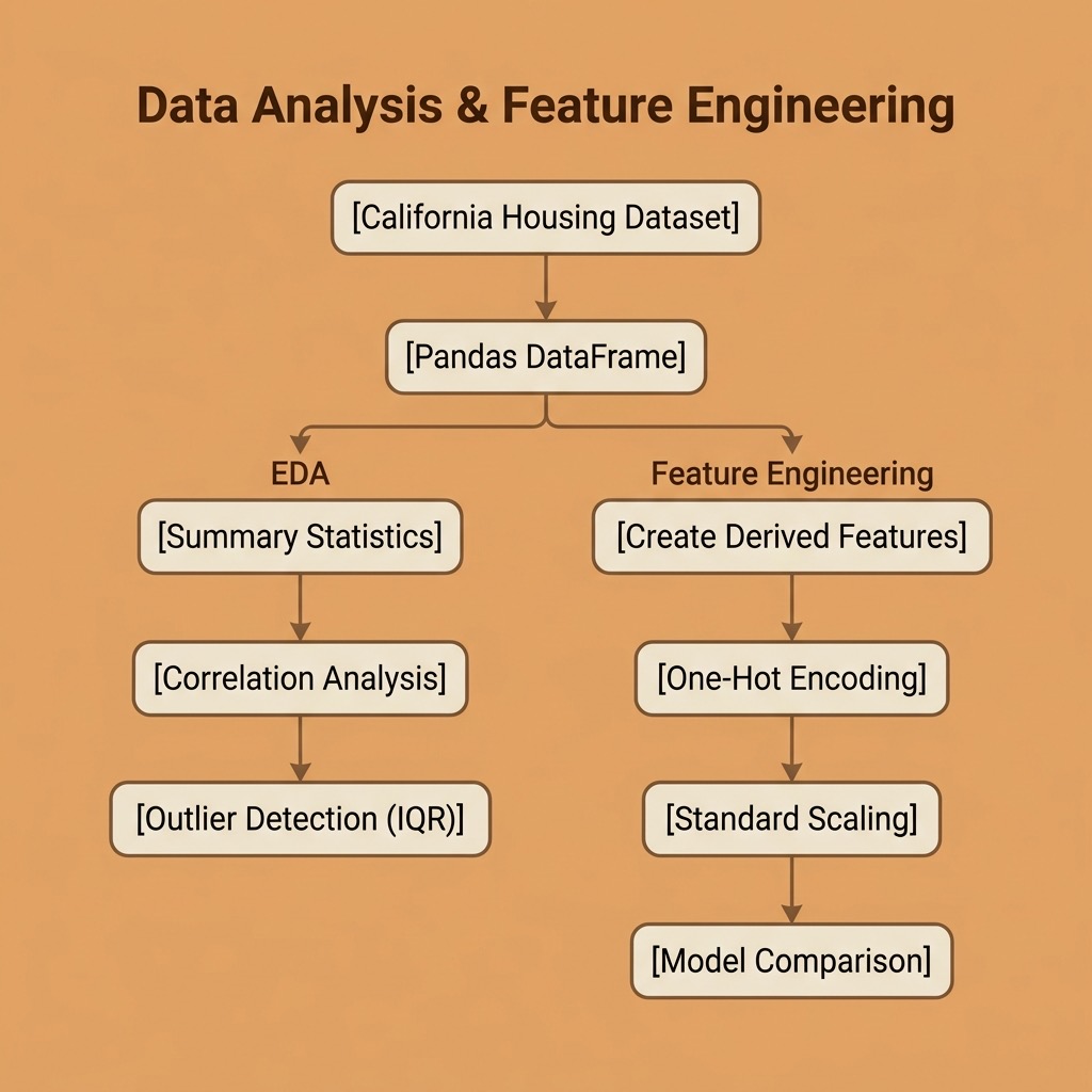
Exploratory Data Analysis and Feature Engineering
Before training any machine learning model, you need to understand your data. Exploratory Data Analysis (EDA) is the process of examining a dataset to summarize its main characteristics, find patterns, detect anomalies, and check assumptions. Feature engineering is the art of creating new input variables — or transforming existing ones — to improve model performance.
These steps often make the difference between a mediocre model and a good one. As the saying goes: “garbage in, garbage out.”
The requirements for this chapter are:
1 uv pip install scikit-learn pandas numpy
The examples for this chapter are in the directory source-code/data_analysis_and_feature_engineering.
We continue using the California Housing dataset from the previous chapter.
Exploratory Data Analysis
Loading and Inspecting the Data
The first thing to do with any dataset is to understand its shape, types, and basic statistics:
 1 import numpy as np
 2 import pandas as pd
 3 from sklearn.datasets import fetch_california_housing
 4
 5 housing = fetch_california_housing()
 6 df = pd.DataFrame(housing.data, columns=housing.feature_names)
 7 df["MedHouseVal"] = housing.target
 8
 9 print(f"Shape: {df.shape[0]} rows × {df.shape[1]} columns")
10 print(df.dtypes)
Running our eda.py script gives us:
 1 $ python eda.py
 2 === Dataset Overview ===
 3 Shape: 20640 rows × 9 columns
 4
 5 Column types:
 6 MedInc         float64
 7 HouseAge       float64
 8 AveRooms       float64
 9 AveBedrms      float64
10 Population     float64
11 AveOccup       float64
12 Latitude       float64
13 Longitude      float64
14 MedHouseVal    float64
All columns are floating point. Next, summary statistics:
1 === Summary Statistics ===
2          MedInc  HouseAge  AveRooms  AveBedrms  Population  AveOccup
3 count  20640.00  20640.00  20640.00   20640.00    20640.00  20640.00
4 mean       3.87     28.64      5.43       1.10     1425.48      3.07
5 std        1.90     12.59      2.47       0.47     1132.46     10.39
6 min        0.50      1.00      0.85       0.33        3.00      0.69
7 max       15.00     52.00    141.91      34.07    35682.00   1243.33
Notice the wide range differences: Population ranges from 3 to 35,682 while AveBedrms ranges from 0.33 to 34.07. This tells us we will need feature scaling before training most models.
Also notice the extreme maximum values for AveRooms (141.91) and AveOccup (1,243.33) — these are likely outliers or data quality issues.
Checking for Missing Values
Missing data can silently break your models or introduce bias. Always check:
1 === Missing Values ===
2 No missing values found.
This dataset is clean, but real-world data rarely is. We will practice handling missing values in the feature engineering section below.
Correlation Analysis
Understanding which features correlate with the target helps guide feature selection and engineering:
1 === Correlation with MedHouseVal ===
2   MedInc                +0.6881
3   AveRooms              +0.1519
4   Latitude              -0.1442
5   HouseAge              +0.1056
6   AveBedrms             -0.0467
7   Longitude             -0.0460
8   Population            -0.0246
9   AveOccup              -0.0237
MedInc (median income) stands out with a correlation of +0.69 — by far the strongest predictor. This aligns with what we saw from the regression coefficients in the previous chapter. The other features have relatively weak linear correlations, suggesting that non-linear relationships or feature combinations might be more informative.
Outlier Detection
The IQR (Interquartile Range) method flags values that fall more than 1.5 × IQR below Q1 or above Q3:
1 === Outlier Counts (IQR method) ===
2   MedInc                  681 outliers (3.3%)
3   AveRooms                511 outliers (2.5%)
4   AveBedrms              1424 outliers (6.9%)
5   Population             1196 outliers (5.8%)
6   AveOccup                711 outliers (3.4%)
7   MedHouseVal            1071 outliers (5.2%)
Nearly 7% of AveBedrms values are outliers. In practice, you would investigate whether these are genuine extreme values or data errors, and decide whether to clip, transform, or remove them depending on your use case.
Feature Engineering
Feature engineering is where domain knowledge meets data science. By creating new features that better represent the underlying patterns, we can significantly improve model performance — sometimes more than choosing a fancier algorithm.
Creating New Features
We can derive meaningful features by combining existing ones:
1 df["RoomsPerHousehold"] = df["AveRooms"] / df["AveOccup"]
2 df["BedroomRatio"] = df["AveBedrms"] / df["AveRooms"]
3 df["PopPerHousehold"] = df["Population"] / df["HouseAge"]
- RoomsPerHousehold: a proxy for house size relative to occupancy.
- BedroomRatio: what fraction of rooms are bedrooms (a measure of house layout).
- PopPerHousehold: population growth rate proxy (newer areas with high population).
Encoding Categorical Features
Many real-world datasets contain categorical variables (e.g., “color”, “region”, “type”). Most ML algorithms require numerical inputs, so we need to encode these.
In our example, we create a categorical feature by binning latitude into California regions, then one-hot encode it:
1 df["Region"] = pd.cut(
2     df["Latitude"],
3     bins=[32, 35, 38, 42],
4     labels=["South", "Central", "North"]
5 )
6
7 region_dummies = pd.get_dummies(df["Region"], prefix="Region", dtype=int)
8 df = pd.concat([df, region_dummies], axis=1)
1 === Region Distribution ===
2 Region
3 South      11294
4 Central     6331
5 North       3015
One-hot encoding creates a separate binary column for each category (Region_South, Region_Central, Region_North). This avoids imposing a false numerical ordering on the categories.
Handling Missing Data
Real datasets almost always have missing values. Common strategies include:
- Drop rows: simple but loses data.
- Fill with mean/median: preserves dataset size; median is more robust to outliers.
- Fill with a model prediction: more sophisticated but adds complexity.
We demonstrate median imputation:
1 # Simulate 5% missing values
2 rng = np.random.default_rng(42)
3 mask = rng.random(len(df)) < 0.05
4 df.loc[mask, "PopPerHousehold"] = np.nan
5
6 # Fill with median
7 median_val = df["PopPerHousehold"].median()
8 df["PopPerHousehold"] = df["PopPerHousehold"].fillna(median_val)
1 === Handling Missing Data ===
2 Introduced 1028 missing values in PopPerHousehold
3 Filled with median: 41.833
4 Remaining missing: 0
Feature Scaling
Features on vastly different scales cause problems for distance-based algorithms (K-NN, K-Means) and gradient-based optimizers. StandardScaler transforms each feature to have zero mean and unit variance:
1 === Feature Scaling Impact ===
2 Before scaling:
3   MedInc           mean=      3.87  std=      1.90
4   AveRooms         mean=      5.43  std=      2.47
5   Population       mean=   1425.48  std=   1132.46
6 After StandardScaler:
7   MedInc           mean=    0.0000  std=    1.0000
8   AveRooms         mean=    0.0000  std=    1.0000
9   Population       mean=   -0.0000  std=    1.0000
After scaling, all features are on the same footing. Remember to always fit the scaler on training data only and apply it to both train and test sets to prevent data leakage.
Measuring the Impact
The ultimate test of feature engineering is whether it improves model performance. We compare a Linear Regression model with the original 8 features against one with our 14 engineered features:
1 === Model Comparison: Original vs. Engineered Features ===
2   Original (8 features)           R² = 0.5758
3   Engineered (14 features)        R² = 0.6622
Our engineered features improved R² from 0.58 to 0.66 — a 15% improvement in explained variance, using the exact same algorithm. This demonstrates why feature engineering is often more valuable than model selection for improving results.
EDA and Feature Engineering Wrap-up
In this chapter we covered the essential data preparation skills that precede model training:
- EDA helps you understand your data through summary statistics, correlation analysis, and outlier detection. Never skip this step.
- Feature engineering transforms raw data into more informative inputs: creating derived features, encoding categories, handling missing values, and scaling.
- The payoff is real: our engineered features produced a 15% improvement in model performance with zero algorithm changes.
These techniques apply to every machine learning project, whether you are using classic algorithms from scikit-learn or deep learning frameworks. In the next part of this book, we move into deep learning.
Optional Practice Problems
To solidify your understanding of exploratory data analysis and feature engineering, try the following practical exercises. You can implement these by modifying or extending the code in source-code/data_analysis_and_feature_engineering/.
1. Outlier Handling: Clipping vs. Dropping (Easy)
In eda.py, we identified that variables like AveRooms and AveOccup have extreme outliers.
- Your Task: Write a function that uses the IQR method (or a fixed percentile threshold, e.g., the 1st and 99th percentiles) to clip (cap and floor) the extreme outliers of these features.
- Extension: Train the linear regression model using these clipped features and compare the
 score against the baseline model. Does outlier clipping improve performance? How does it compare to dropping rows with outliers?
2. Evaluating Alternative Scaling Methods (Medium)
Our code uses StandardScaler to normalize features. However, features with large outliers can distort the mean and standard deviation.
- Your Task: Update
feature_engineering.pyto compare three different scaling methods fromsklearn.preprocessing:StandardScaler,MinMaxScaler, andRobustScaler. - Extension: Evaluate the linear regression model’s score under each scaling method. Analyze the results: which scaler is more robust to extreme values, and how do they affect the final regression model?
3. Geographic Feature Engineering with Clustering (Hard)
The coordinates Latitude and Longitude represent spatial locations, but binning latitude into three simple regions (North, Central, South) ignores local cluster densities (such as the San Francisco Bay Area and Greater Los Angeles).
- Your Task: Implement a script that uses the
KMeansalgorithm fromsklearn.clusterto group coordinates into spatial clusters (e.g.,
  ).
).
- Extension: Use the distance from each housing block to the cluster centers (obtained using
kmeans.transform(coordinates)) as new continuous features, or one-hot encode the cluster assignments. Train the linear regression model with these clustering-based geographic features and compare the score against the simple regional binning approach.