Regression and Clustering
In the previous chapter we used a K-Nearest Neighbors classifier with scikit-learn. Here we expand our coverage of “classic” machine learning with two more fundamental techniques: regression for predicting continuous values, and clustering for discovering groups in data without labeled targets.
The requirements for this chapter are:
1 uv pip install scikit-learn pandas numpy
The examples for this chapter are in the directory source-code/regression_and_clustering.
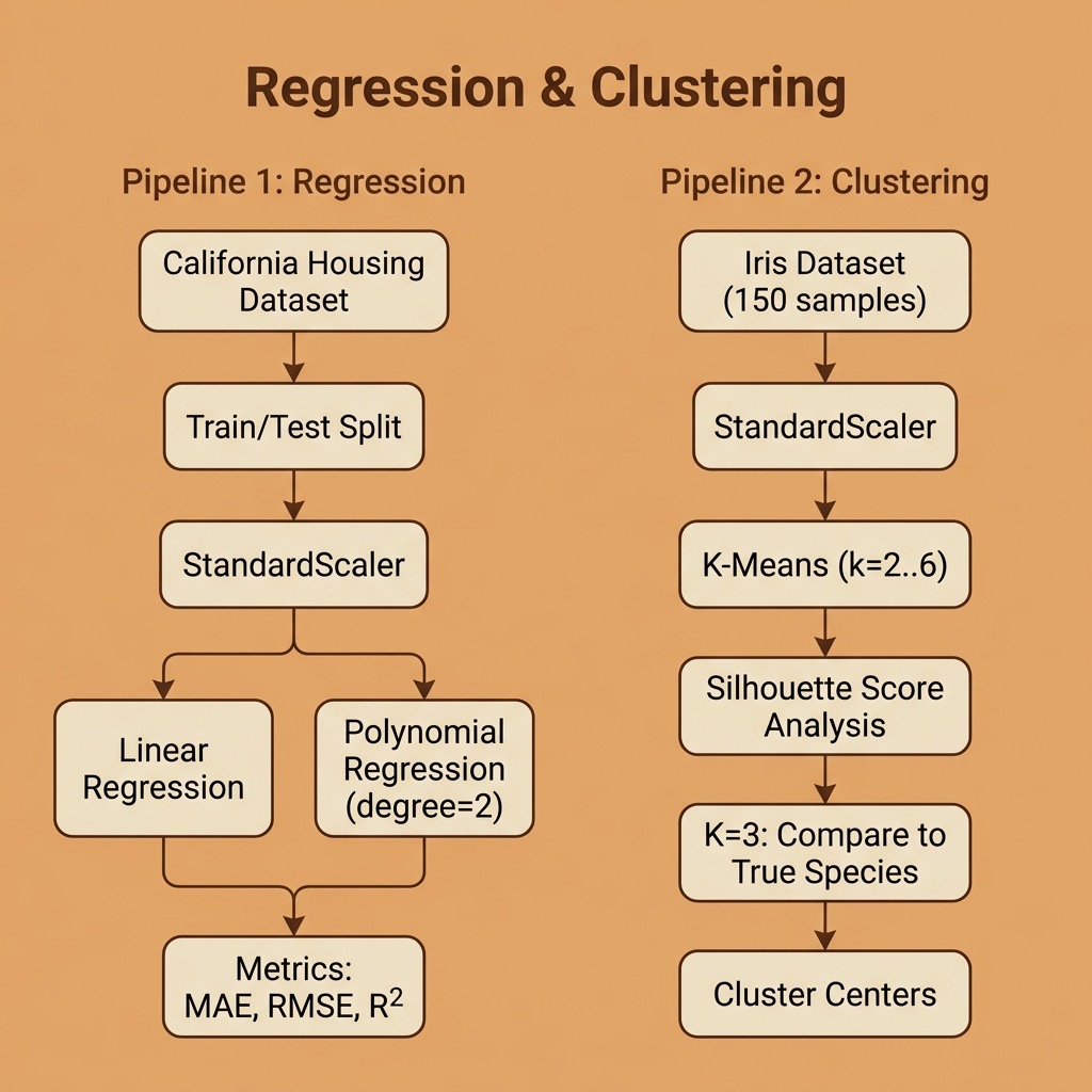
Regression: Predicting Housing Prices
Regression is a type of supervised machine learning where the goal is to predict a continuous numerical value rather than a class label. While classification asks “which category?”, regression asks “how much?” or “how many?”
Common regression algorithms include:
- Linear Regression: models the relationship between features and target as a straight line (or hyperplane in multiple dimensions).
- Polynomial Regression: extends linear regression by adding polynomial terms, allowing the model to capture non-linear relationships.
- Ridge and Lasso Regression: variants of linear regression that add regularization to prevent overfitting.
We will use the California Housing dataset, which is built into scikit-learn. It contains 20,640 samples with 8 features describing California census block groups (median income, average number of rooms, location, etc.), with the target being the median house value in units of $100,000s.
Linear Regression
Our first example fits a linear regression model to all 8 features:
 1 import numpy as np
 2 import pandas as pd
 3 from sklearn.datasets import fetch_california_housing
 4 from sklearn.linear_model import LinearRegression
 5 from sklearn.preprocessing import PolynomialFeatures, StandardScaler
 6 from sklearn.metrics import mean_absolute_error, mean_squared_error, r2_score
 7 from sklearn.model_selection import train_test_split
 8
 9
10 def load_housing_data():
11     """Load the California Housing dataset into a DataFrame."""
12     housing = fetch_california_housing()
13     df = pd.DataFrame(housing.data, columns=housing.feature_names)
14     df["MedHouseVal"] = housing.target
15     return df
We use train_test_split to hold out 20% of the data for evaluation, scale the features with StandardScaler, and train the model:
 1 df = load_housing_data()
 2 X = df.drop("MedHouseVal", axis=1)
 3 y = df["MedHouseVal"]
 4
 5 X_train, X_test, y_train, y_test = train_test_split(
 6     X, y, test_size=0.2, random_state=42
 7 )
 8
 9 scaler = StandardScaler()
10 X_train_scaled = scaler.fit_transform(X_train)
11 X_test_scaled = scaler.transform(X_test)
12
13 model = LinearRegression()
14 model.fit(X_train_scaled, y_train)
15 y_pred = model.predict(X_test_scaled)
To evaluate a regression model, we use different metrics than classification:
- MAE (Mean Absolute Error): average magnitude of prediction errors in the same units as the target.
- RMSE (Root Mean Squared Error): like MAE but penalizes larger errors more heavily.
- R² (R-squared): the proportion of variance in the target explained by the model (1.0 = perfect, 0.0 = no better than predicting the mean).
Here is the output of running the full regression.py script:
 1 $ python regression.py
 2 Dataset shape: (20640, 9)
 3 Target range: 0.15 - 5.00 (units: $100,000s)
 4
 5 === Linear Regression Results ===
 6   MAE:  0.5332
 7   RMSE: 0.7456
 8   R²:   0.5758
 9
10 Feature coefficients (scaled):
11   MedInc               +0.8544
12   HouseAge             +0.1225
13   AveRooms             -0.2944
14   AveBedrms            +0.3393
15   Population           -0.0023
16   AveOccup             -0.0408
17   Latitude             -0.8969
18   Longitude            -0.8698
Because we scaled the features, the coefficients tell us the relative importance of each feature. MedInc (median income) has the largest positive coefficient, confirming that income is the strongest predictor of housing prices. The geographic features (Latitude and Longitude) are also very influential — location matters!
An R² of 0.58 means our simple linear model explains about 58% of the variance in housing prices. Not bad for a single line of model code, but there is room for improvement.
Polynomial Regression
We can capture non-linear relationships by creating polynomial features. For interpretability, we use just two features (MedInc and AveRooms) and generate all degree-2 combinations:
1 poly = PolynomialFeatures(degree=2, include_bias=False)
2 X_train_poly = poly.fit_transform(X_train_scaled)
3 X_test_poly = poly.transform(X_test_scaled)
4
5 model = LinearRegression()
6 model.fit(X_train_poly, y_train)
The PolynomialFeatures transformer with degree=2 creates five features from our original two: x0, x1, x0², x0·x1, and x1². The interaction term x0·x1 lets the model learn that the relationship between income and price depends on the number of rooms.
1 === Polynomial Regression (degree=2, 2 features) ===
2   MAE:  0.6163
3   RMSE: 0.8402
4   R²:   0.4613
5
6   Polynomial feature names: ['x0', 'x1', 'x0^2', 'x0 x1', 'x1^2']
With only 2 features, the polynomial model achieves R²=0.46 compared to 0.58 with all 8 features linearly. This illustrates an important tradeoff: polynomial features add expressive power but using too few input features limits the information available to the model.
Clustering: Discovering Groups in Data
Clustering is an unsupervised learning technique — unlike classification and regression, we do not provide labeled targets. Instead, the algorithm discovers natural groupings in the data.
K-Means is the most widely used clustering algorithm. It works by:
- Choosing K initial cluster centers (centroids).
- Assigning each data point to the nearest centroid.
- Recomputing each centroid as the mean of its assigned points.
- Repeating steps 2-3 until convergence.
We will use the classic Iris dataset (150 samples, 4 features measuring sepal and petal dimensions, with 3 known species). This lets us evaluate how well K-Means recovers the true species groupings.
Choosing K with the Silhouette Score
A common question is: how many clusters should we use? The silhouette score measures how similar each point is to its own cluster compared to other clusters (ranging from -1 to +1, higher is better):
 1 from sklearn.cluster import KMeans
 2 from sklearn.preprocessing import StandardScaler
 3 from sklearn.metrics import silhouette_score
 4
 5 scaler = StandardScaler()
 6 X_scaled = scaler.fit_transform(X)
 7
 8 for k in range(2, 7):
 9     km = KMeans(n_clusters=k, random_state=42, n_init=10)
10     labels = km.fit_predict(X_scaled)
11     score = silhouette_score(X_scaled, labels)
12     print(f"  k={k}: silhouette score = {score:.4f}")
Output from running clustering.py:
 1 $ python clustering.py
 2 Dataset: 150 samples, 4 features
 3 Features: ['sepal length (cm)', 'sepal width (cm)',
 4            'petal length (cm)', 'petal width (cm)']
 5 Known species: ['setosa', 'versicolor', 'virginica']
 6
 7 === Silhouette Scores for Different k Values ===
 8   k=2: silhouette score = 0.5818
 9   k=3: silhouette score = 0.4599
10   k=4: silhouette score = 0.3869
11   k=5: silhouette score = 0.3459
12   k=6: silhouette score = 0.3171
The silhouette score is highest at k=2, which suggests that the data most naturally splits into two groups. This makes biological sense: setosa is very distinct from the other two species, while versicolor and virginica overlap considerably.
Comparing Clusters to True Labels
Since we happen to know the true species labels, we can use a cross-tabulation to see how well K-Means (with k=3) recovers them:
1 === K-Means (k=3) Cluster vs. True Species ===
2 Cluster      0   1   2
3 Species
4 setosa       0  50   0
5 versicolor  39   0  11
6 virginica   14   0  36
K-Means perfectly separates all 50 setosa samples into cluster 1. However, it struggles to distinguish versicolor from virginica — 14 virginica samples are assigned to the versicolor-dominant cluster 0, and 11 versicolor samples end up in the virginica-dominant cluster 2. This confirms what the silhouette scores suggested.
The cluster centers (transformed back to the original scale) reveal the “typical” flower in each group:
1 === Cluster Centers (original scale) ===
2          sepal length  sepal width  petal length  petal width
3 Cluster
4 0                5.80         2.67          4.37         1.41
5 1                5.01         3.43          1.46         0.25
6 2                6.78         3.10          5.51         1.97
Cluster 1 (setosa) has much smaller petals, while cluster 2 (mostly virginica) has the largest sepals and petals.
Regression and Clustering Wrap-up
In this chapter we covered two fundamental machine learning techniques beyond classification:
- Regression lets us predict continuous values. We saw that even simple linear regression can be informative, and that feature coefficients reveal which inputs drive predictions.
- Clustering discovers structure in unlabeled data. We used silhouette scores to evaluate cluster quality and cross-tabulations to compare clusters against known labels.
Together with the classification example in the previous chapter, you now have hands-on experience with the three core tasks of classic machine learning. In the next chapter we will explore the data preparation work that comes before training any model.
Optional Practice Problems
To solidify your understanding of regression and clustering, try these practical exercises. They build upon the code examples in the source-code/regression_and_clustering directory.
1. The Impact of Feature Scaling on Clustering (Easy)
Distance-based algorithms like K-Means are highly sensitive to the scale of the input features.
- Task: Modify
clustering.pyto run K-Means on the original, unscaled datasetX(instead ofX_scaled). -
Requirements:
- Calculate and print the silhouette scores for
 through
  using the unscaled data.
- Generate a cross-tabulation table comparing clusters (
 ) to the true species labels for the unscaled model.
- Questions for Reflection: How do the silhouette scores change when scaling is omitted? Looking at the features, why does sepal length or petal length dominate the distance calculations when unscaled?
2. Ridge and Lasso Regularization (Medium)
Standard Linear Regression can overfit or behave erratically when features are correlated. Regularization adds a penalty term to shrink coefficients.
- Task: Extend
regression.pyto train and evaluateRidgeandLassomodels fromsklearn.linear_modelon the California Housing dataset. -
Requirements:
- Train
RidgeandLassomodels using all 8 features (using scaled training data). - Compare their metrics (MAE, RMSE,
 ) to the standard
 LinearRegressionmodel. - Print the feature coefficients for all three models side-by-side. Experiment with different regularization strengths (
alpha=0.1,alpha=1.0,alpha=10.0).
- Questions for Reflection: What is the key difference between Ridge (L2 penalty) and Lasso (L1 penalty) regarding the sparsity of the coefficients? Which coefficients shrink to exactly zero first under Lasso?
3. Choosing k with the Elbow Method (Medium)
While the silhouette score is a powerful metric, the “Elbow Method” using the sum of squared distances to the nearest centroid (inertia) is also widely used.
- Task: Write a short script or modify
clustering.pyto implement the Elbow Method. -
Requirements:
- Run K-Means on the scaled Iris dataset for
 values from
  to
to  .
.
- Record the value of the
inertia_attribute for each.
- Print or plot the relationship between and inertia.
- Questions for Reflection: Identify the “elbow” point where the rate of decrease in inertia slows down significantly. Does this elbow match the optimal cluster count suggested by the silhouette score?
4. Robust Tuning with Pipelines and Grid Search (Hard)
Evaluating hyperparameter tuning and preprocessing choices using a single train/test split can lead to data leakage and overly optimistic metrics. A better approach is to wrap preprocessing and modeling steps in a pipeline and use cross-validation.
- Task: Create a new script,
housing_pipeline.py, in your source code directory. -
Requirements:
- Define a scikit-learn
PipelinecontainingStandardScaler,PolynomialFeatures(include_bias=False), andRidge. -
Use
GridSearchCVwith 5-fold cross-validation to search over a grid of:- Polynomial degree:
[1, 2] - Ridge parameter
alpha:[0.1, 1.0, 10.0, 100.0]
- Print the best parameters found by the grid search.
- Evaluate the best estimator on your held-out test set and report the final MAE, RMSE, and.
- Questions for Reflection: Why is it important to put
StandardScalerinside the pipeline rather than scaling the entire dataset before cross-validation? How did the performance of this optimized model compare to the simple OLS model in the chapter?