The Basics of Deep Learning
Deep learning is a subfield of machine learning that is concerned with the design and implementation of artificial neural networks (ANNs) with multiple layers, also known as deep neural networks (DNNs). These networks are inspired by the structure and function of the human brain, and are designed to learn from large amounts of data such as images, text, and audio.
A neural network consists of layers of interconnected nodes, or neurons, which are organized into an input layer, one or more hidden layers, and an output layer. Each neuron receives input from the neurons in the previous layer, performs a computation, and passes the result to the neurons in the next layer. The computation typically involves a dot product of the input with a set of weights and an activation function, which is a non-linear function applied to the result. The weights are the parameters of the network that are learned during training.
The basic building block of a deep neural network is an artificial neuron, also known as perceptron, which is a simple mathematical model for a biological neuron. A perceptron receives input from other neurons and it applies a linear transformation to the input, followed by a non-linear activation function.
Deep learning networks can be feedforward networks where the data flows in one direction from input to output, or recurrent networks where the data can flow in a cyclic fashion.
There are different types of deep learning architectures such as feedforward neural networks, convolutional neural networks (CNNs), recurrent neural networks (RNNs) and Generative Adversarial Networks (GANs). These architectures are designed to learn specific types of features and patterns from different types of data.
Deep learning models are trained using large amounts of labeled data, and typically use supervised or semi-supervised learning techniques. The training process involves adjusting the weights of the network to minimize a loss function, which measures the difference between the predicted output and the true output. This process is known as back-propagation, which is an algorithm for training the weights in a neural network by propagating the error back through the network. In the first AI book I wrote in the 1980s I covered the implementation of back-propagation in detail. As I write the material here on deep learning I think that it is more important for you to have the skills to choose appropriate tools for different applications and be less concerned about low-level implementation details. I think this characterizes the change in trajectory of AI from being about tool building to the skills of using available tools and sometimes previously trained models while spending more of your effort analyzing business functions and in general application domains.
Deep Learning has been applied to various fields such as Computer Vision, Natural Language Processing, Speech Recognition, etc.
Using PyTorch for Building a Cancer Prediction Model
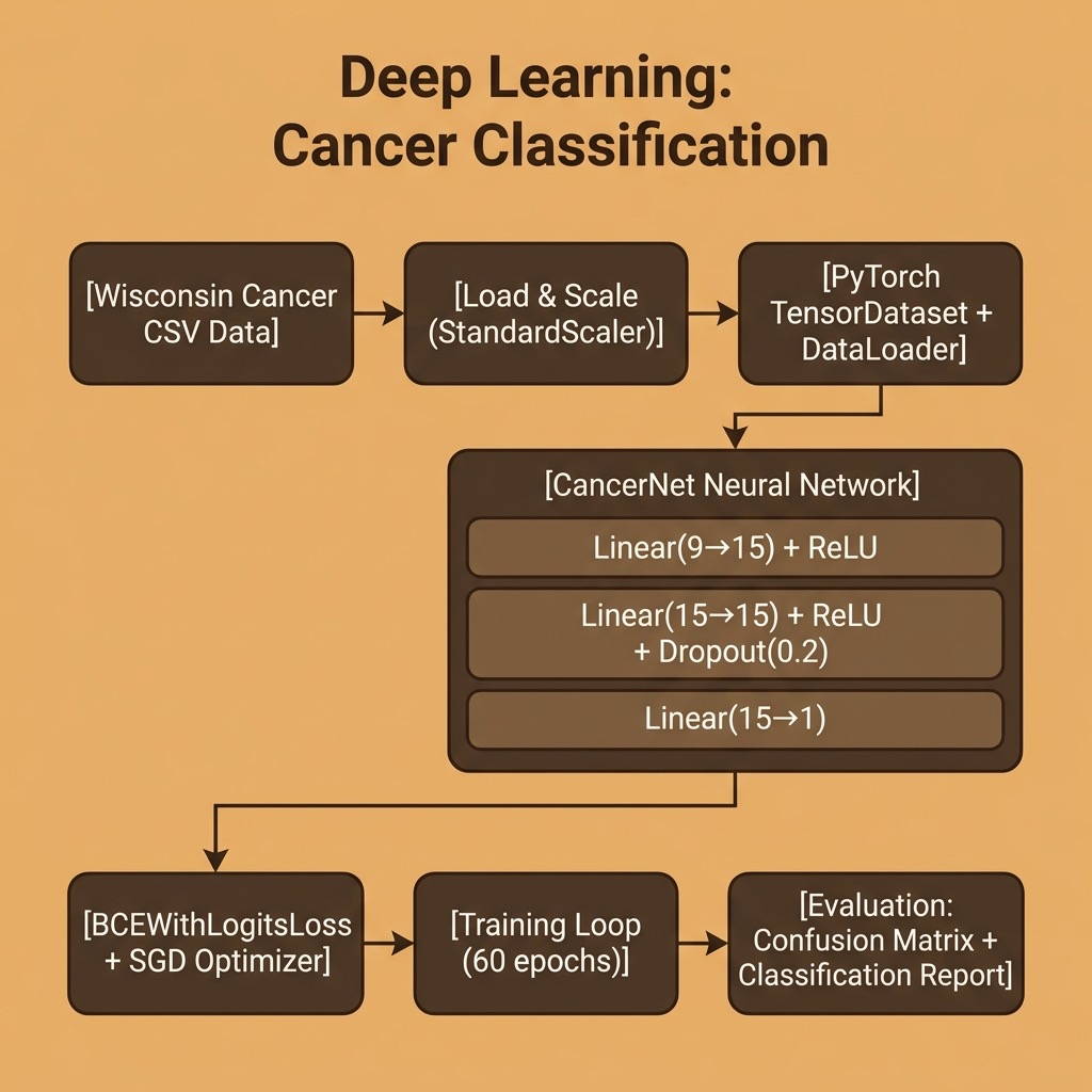
We will use PyTorch to build a neural network that classifies the same University of Wisconsin cancer dataset we used in the scikit-learn chapter. This lets us directly compare the deep learning approach with the classic K-Nearest Neighbors classifier.
The examples for this chapter are in the directory source-code/deep_learning_basics.
The requirements for this chapter are:
1 uv pip install torch scikit-learn pandas numpy
Why PyTorch?
PyTorch is the most widely used deep learning framework in both research and industry. Developed originally by Meta AI, it provides:
- Dynamic computation graphs: build and modify your network on-the-fly, making debugging natural.
- Pythonic API: feels like writing regular Python code, not configuring a separate computation engine.
- Extensive ecosystem: integrates with Hugging Face Transformers, torchvision, torchaudio, and many more libraries.
- Strong GPU support: seamlessly move computations between CPU, CUDA GPUs, and Apple Silicon (MPS).
Loading and Preparing the Data
We reuse the same CSV data files from our machine learning chapter. The data loading code converts the Pandas DataFrames to NumPy arrays, scales the features, then wraps everything in PyTorch tensors:
 1 import numpy as np
 2 import pandas as pd
 3 import torch
 4 import torch.nn as nn
 5 from torch.utils.data import DataLoader, TensorDataset
 6 from sklearn.preprocessing import StandardScaler
 7
 8 def load_data():
 9     """Load the cancer CSV files."""
10     train_df = pd.read_csv("../machine-learning/labeled_cancer_data.csv")
11     test_df = pd.read_csv("../machine-learning/labeled_test_data.csv")
12
13     train = train_df.to_numpy()
14     X_train = train[:, 0:9].astype(np.float32)
15     Y_train = train[:, -1].astype(np.float32).reshape(-1, 1)
16
17     test = test_df.to_numpy()
18     X_test = test[:, 0:9].astype(np.float32)
19     Y_test = test[:, -1].astype(np.float32).reshape(-1, 1)
20
21     scaler = StandardScaler()
22     X_train = scaler.fit_transform(X_train)
23     X_test = scaler.transform(X_test)
24
25     return X_train, Y_train, X_test, Y_test
Note that we use np.float32 — PyTorch expects 32-bit floats by default (unlike NumPy’s default of 64-bit).
Defining the Model
In PyTorch, we define neural network architectures by subclassing nn.Module. Our network has two hidden layers of 15 neurons with ReLU activation, a dropout layer for regularization, and a single output neuron:
 1 class CancerNet(nn.Module):
 2     """Simple feedforward network: 9 → 15 → 15 → 1."""
 3
 4     def __init__(self):
 5         super().__init__()
 6         self.network = nn.Sequential(
 7             nn.Linear(9, 15),
 8             nn.ReLU(),
 9             nn.Linear(15, 15),
10             nn.ReLU(),
11             nn.Dropout(0.2),
12             nn.Linear(15, 1),
13         )
14
15     def forward(self, x):
16         return self.network(x)
The forward method defines how data flows through the network. PyTorch’s autograd system automatically computes the gradients needed for backpropagation — we never need to write the backward pass manually.
The Training Loop
Unlike higher-level frameworks, PyTorch gives you explicit control over the training loop. This makes it easy to customize training behavior, add logging, or implement complex training schedules:
 1 def train_model(model, train_loader, epochs=60, lr=0.01):
 2     criterion = nn.BCEWithLogitsLoss()
 3     optimizer = torch.optim.SGD(model.parameters(), lr=lr)
 4
 5     for epoch in range(epochs):
 6         total_loss = 0.0
 7         for X_batch, y_batch in train_loader:
 8             optimizer.zero_grad()
 9             outputs = model(X_batch)
10             loss = criterion(outputs, y_batch)
11             loss.backward()
12             optimizer.step()
13             total_loss += loss.item()
14
15         if (epoch + 1) % 10 == 0:
16             avg_loss = total_loss / len(train_loader)
17             print(f"  Epoch {epoch+1:3d}/{epochs}  loss: {avg_loss:.4f}")
We use BCEWithLogitsLoss which combines a sigmoid activation with binary cross-entropy loss — this is numerically more stable than applying sigmoid separately. The training loop follows the standard PyTorch pattern: zero gradients, forward pass, compute loss, backward pass, update weights.
Running the Example
Here is the complete output from running cancer_model.py:
 1 $ python cancer_model.py
 2 Training examples: 554
 3 Test examples:     15
 4
 5 CancerNet(
 6   (network): Sequential(
 7     (0): Linear(in_features=9, out_features=15, bias=True)
 8     (1): ReLU()
 9     (2): Linear(in_features=15, out_features=15, bias=True)
10     (3): ReLU()
11     (4): Dropout(p=0.2, inplace=False)
12     (5): Linear(in_features=15, out_features=1, bias=True)
13   )
14 )
15
16 Training:
17   Epoch  10/60  loss: 0.6913
18   Epoch  20/60  loss: 0.6559
19   Epoch  30/60  loss: 0.6250
20   Epoch  40/60  loss: 0.5874
21   Epoch  50/60  loss: 0.5421
22   Epoch  60/60  loss: 0.4969
23
24 Confusion Matrix:
25 [[9 0]
26  [1 5]]
27
28 Classification Report:
29               precision    recall  f1-score   support
30
31          0.0       0.90      1.00      0.95         9
32          1.0       1.00      0.83      0.91         6
33
34     accuracy                           0.93        15
35    macro avg       0.95      0.92      0.93        15
36 weighted avg       0.94      0.93      0.93        15
37
38 Sample predictions (should be close to [[0], [1]]):
39 [[0.8588059]
40  [0.9907742]]
The model achieves 93% accuracy on the test set — matching the performance of our scikit-learn KNN classifier from the earlier chapter. The loss decreases steadily during training, and the sample predictions show that the model learns to distinguish between non-malignant and malignant cases.
You can compare this PyTorch example to our similar classification example using the same data where we used the Scikit-learn library. The deep learning approach requires more code but gives us full control over the model architecture, training process, and the ability to scale to much larger and more complex problems.
Optional Practice Problems
To help solidify your understanding of deep learning basics and PyTorch, try completing the following exercises. You will need to modify and run the example script cancer_model.py.
Problem 1 (Easy): Experimenting with Optimizers and Learning Rates
- Goal: Understand how optimizer choice and learning rate affect training speed and model convergence.
- Task: Modify cancer_model.py to use the Adam optimizer (
torch.optim.Adam) instead of Stochastic Gradient Descent (torch.optim.SGD). Experiment with three different learning rates (e.g.,0.1,0.01, and0.001). Note down how quickly the loss decreases during training and how the final test set accuracy is affected. Which combination reaches convergence first?
Problem 2 (Medium): Implementing Validation Tracking and Overfitting Analysis
- Goal: Learn how to monitor validation performance during training to detect overfitting.
- Task: Split the training data further into training and validation sets (using a 80/20 split). Modify the train_model function to evaluate the model on the validation set at the end of each epoch and track both the average training loss and validation loss. Print a table (or use
matplotlibto plot) showing the two loss curves across 150 epochs. At what epoch does the validation loss start to diverge or stop decreasing?
Problem 3 (Medium): Adjusting Network Architecture and Regularization
- Goal: Understand the role of network capacity (hidden layers/neurons) and regularization (dropout).
-
Task: Modify the architecture in the CancerNet class. Try two variations:
- A much smaller network with a single hidden layer and no dropout:
9 → 5 → 1. - A larger network with more capacity:
9 → 32 → 32 → 1with varying dropout rates (0.0,0.2, and0.5). Analyze the classification report for both cases. How does the presence of dropout in the larger network affect the performance gap between the training set loss and the test set accuracy?
Problem 4 (Hard): Implementing K-Fold Cross-Validation
- Goal: Practice using robust evaluation techniques for small datasets.
- Task: Since the cancer dataset is relatively small, a single train/test split can have high variance. Instead of a single split, implement 5-Fold Cross-Validation using
sklearn.model_selection.KFoldin cancer_model.py. In each fold, initialize a new instance of CancerNet, train it, and evaluate it on the holdout fold. Compute and print the average accuracy, precision, recall, and F1-score across all 5 folds.