Categorical Deep Learning: From Axioms to Implementation using Category Theory
Earlier in this book we built neural networks with PyTorch and let its autograd system handle backpropagation for us. That is the right approach for production work. In this chapter I want to take you in the opposite direction: we will build a complete deep learning framework from scratch using only the Python standard library, and we will see that the structure of backpropagation, dropout, Bayesian uncertainty, ensemble consistency, and knowledge distillation all fall out naturally from the language of category theory.
The inspiration for this chapter is the survey paper by Jia, Peng, Yang and Chen (2025), “Category-Theoretical and Topos-Theoretical Frameworks in Machine Learning: A Survey” (Axioms 14(3):204). The paper organizes categorical machine learning into five perspectives, and we will implement all five in a single Python file with no external dependencies. If you have never studied category theory, do not worry: I will introduce each concept just before we use it, and the code is the real teacher here.
In the context of the Para category, a morphism is a parameterized, bidirectional mapping structure known as a lens. A neural network layer is not a simple map from A->B. It is a morphism defined as a triple (P,F,F*):
- P: The parameter space (weights and biases).
- F: The forward pass mapping parameters and inputs to outputs.
- F∗: The pullback (backward pass) mapping upstream gradients back to parameter and input gradients.
Calling a layer a “morphism in the Para category” means the layer is a single, self-contained mathematical unit that inherently contains both its forward execution and its exact backpropagation mechanism.
Why bother with category theory when PyTorch and TensorFlow already work and have been tuned for high efficiency on GPUs and TPUs? Because the categorical viewpoint reveals why neural networks are structured the way they are. When you see that a neural network layer is a morphism in the Para category, that backpropagation is the composition of pullback morphisms, and that a sigmoid output is a subobject classifier in a topos, you gain a deeper understanding that transfers to new architectures and new problems. I have found that this perspective makes me a better engineer even when I never write a custom framework in production.
The examples for this chapter are in the directory source-code/deep_learning_category_theory.
This example uses only the Python standard library (math and random), so there is nothing to install:
1 uv run deep_learning_category_theory.py
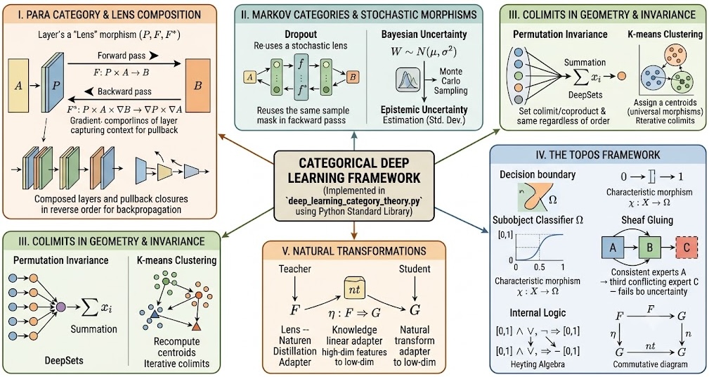
The Para Category and Lens Composition
Traditional backpropagation is often taught as a sequence of calculus rules applied by hand. Categorical deep learning views it more profoundly: layers are morphisms in the Para category, which is specifically designed to handle parametric maps between states.
In the Para construction, a morphism f : A -> B is a triple (P, F, F*), where:
- P is the parameter space (the weights and biases for one layer).
F: P × A -> Bis the forward pass, mapping parameters and input to output.F*: P × A × dB -> dP × dAis the pullback (backward pass), which computes how infinitesimal changes in the outputdBpropagate back into parameter spacedPand input spacedA.
The key insight is that a neural network layer is not just a function. It is a bidirectional structure: a forward map paired with a backward map. Category theorists call this a lens. The forward half produces output and stashes away enough context to run the backward half later. The backward half receives a gradient from upstream and produces gradients for both the parameters and the input.
Implementing a Para Morphism
In our implementation, LayerParams represents an object in the parameter space, and the function forward_para realizes a morphism in Para(Euc):
 1 def forward_para(
 2     params: LayerParams,
 3     act: Callable[[float], float],
 4     act_deriv: Callable[[float], float],
 5     inputs: list[float],
 6 ) -> tuple[list[float], PullbackFn]:
 7     W = params.W
 8     b = params.b
 9     zs = vec_add(matvec(W, inputs), b)   # pre-activations
10     acts = [act(z) for z in zs]           # post-activations
11
12     def pullback(upstream_grad: list[float]) -> tuple[LayerGrads, list[float]]:
13         delta = [u * act_deriv(z) for u, z in zip(upstream_grad, zs)]
14         dW = outer(delta, inputs)
15         db = list(delta)
16         dx = matT_vec(W, delta)
17         return LayerGrads(dW=dW, db=db), dx
18
19     return acts, pullback
The function returns two things: the post-activation output vector and a pullback closure. The closure captures W, inputs, and zs (the pre-activations) so that when it is called later with an upstream gradient, it can compute the weight gradient dW = δ ⊗ xᵀ, the bias gradient db = δ, and the input gradient dx = Wᵀ · δ that gets passed to the previous layer. This closure is the “put-back” half of the categorical lens.
Compositional Backpropagation
One of the key results of the categorical framework is that neural networks are simply the composition of Para morphisms. If we have layers f₁, f₂, …, fₙ, the cumulative forward effect is:
Fnet = fₙ ∘ f(n-1) ∘ … ∘ f₁
The backward pass composes the pullback morphisms in reverse order:
f₁* ∘ f₂* ∘ … ∘ fₙ* : dŶ -> (dP₁, …, dPₙ, dX)
This is implemented in model_backward, which iterates over the list of pullback closures in reverse, threading the gradient through each layer:
1 def model_backward(pullbacks: list[PullbackFn], dl_dy_hat: float) -> list[LayerGrads]:
2     upstream: list[float] = [dl_dy_hat]
3     grads_acc: list[LayerGrads] = []
4
5     for pb in reversed(pullbacks):
6         grads, upstream = pb(upstream)
7         grads_acc.append(grads)
8
9     return list(reversed(grads_acc))
The SGD update step θ <- θ − η dθ is an endomorphism u_η : Model -> Model on the parameter object. Training is just iterated application of this endomorphism over the dataset.
Demo: Learning XOR
We test the framework on the classic XOR problem, using a network with architecture input(2) -> hidden(4) -> hidden(4) -> output(1) trained for 6000 epochs:
1 xor_data: list[tuple[InputVec, TargetVal]] = [
2     (InputVec(vals=(0.0, 0.0)), TargetVal(v=0.0)),
3     (InputVec(vals=(0.0, 1.0)), TargetVal(v=1.0)),
4     (InputVec(vals=(1.0, 0.0)), TargetVal(v=1.0)),
5     (InputVec(vals=(1.0, 1.0)), TargetVal(v=0.0)),
6 ]
7
8 xor_model = make_network([(2, 4), (4, 4), (4, 1)])
9 trained_xor = train(xor_model, xor_data, eta=0.5, epochs=6000, print_every=2000)
Here is the output from running the demo:
 1 ---  I. Para Category + Lens Composition  (XOR problem)  ---
 2   Architecture: input(2) -> hidden(4) -> hidden(4) -> output(1)
 3   Para morphisms composed sequentially; pullbacks in reverse.
 4
 5   Epoch 0  loss: 1.179186
 6   Epoch 2000  loss: 0.007290
 7   Epoch 4000  loss: 0.001281
 8   -> Predictions after 6000 epochs:
 9       Input: [0.0, 0.0]  Target: 0.0  Pred: 0.0095  Class: 0
10       Input: [0.0, 1.0]  Target: 1.0  Pred: 0.9922  Class: 1
11       Input: [1.0, 0.0]  Target: 1.0  Pred: 0.9819  Class: 1
12       Input: [1.0, 1.0]  Target: 0.0  Pred: 0.0139  Class: 0
The network learns XOR perfectly. What is notable is that we wrote the entire backpropagation mechanism by composing pullback closures, with no autograd library and no calculus rules applied by hand in the training loop. The categorical structure did the work for us.
Markov Categories and Stochastic Morphisms
Machine learning is inherently stochastic. Dropout randomly zeroes neurons, Bayesian weights are sampled from distributions, and training data is shuffled. We model this with Markov categories, where morphisms represent stochastic kernels that map objects to probability distributions over other objects.
A Markov category is a symmetric monoidal category where every object X carries a comonoid structure: a copy map X -> X (x) X where (x) represents a tensor product (duplication) and a delete map X -> I (marginalization). Morphisms are stochastic kernels. In practice, we represent a stochastic morphism as a function that samples an output each time it is called.
Dropout as a Stochastic Lens
Dropout can be formalized as a stochastic lens. The forward pass samples a Bernoulli mask and applies it to the activations. The backward pass must reuse the same mask. This sharing of random state between forward and backward passes is what category theorists call the “closed” lens requirement.
 1 def make_dropout_lens(keep_prob: float):
 2     def dropout_forward(inputs: list[float]):
 3         mask = [1.0 if random.random() < keep_prob else 0.0 for _ in inputs]
 4         scale = 1.0 / keep_prob
 5         masked = [x * m * scale for x, m in zip(inputs, mask)]
 6
 7         def pullback(upstream: list[float]) -> list[float]:
 8             return [u * m * scale for u, m in zip(upstream, mask)]
 9
10         return masked, pullback
11
12     return dropout_forward
The scale factor implements inverted dropout, which keeps the expected activation constant regardless of the keep probability. The pullback closure reuses the exact same mask sampled during the forward pass, ensuring mathematical consistency between the stochastic forward pass and the deterministic gradient flow.
Bayesian Uncertainty via Monte Carlo Sampling
In a Bayesian neural network, weights are treated as random variables W ∼ p(W). A single layer becomes a stochastic morphism: instead of using fixed weights, it samples from a distribution at every forward pass. We implement this with bayesian_forward, which samples weights from a Gaussian W is sample from N(μ, σ²) each time it is called.
By running Monte Carlo sampling (multiple stochastic forward passes), we can compute the empirical mean and standard deviation of the predictions. The standard deviation quantifies epistemic uncertainty, which is the model’s uncertainty about its own parameterization:
1 def bayesian_predict_mc(bl: BayesianLayer, inputs: list[float], n_samples: int):
2     samples = [bayesian_forward(bl, inputs)[0] for _ in range(n_samples)]
3     mean = sum(samples) / n_samples
4     variance = sum((s - mean) ** 2 for s in samples) / n_samples
5     return mean, math.sqrt(variance)
Here is the output from the stochastic morphisms demo:
 1 ━━━━  II. Markov Categories - Stochastic Morphisms  ━━━━
 2
 3   II-A  Dropout (stochastic lens, Bernoulli(0.7) mask)
 4     Input:       [1.0, 2.0, 3.0, 4.0, 5.0]
 5     After drop:  ['0.000', '2.857', '0.000', '0.000', '7.143']
 6     Grad (back): ['0.000', '1.429', '0.000', '0.000', '1.429']
 7
 8   II-B  Bayesian layer - Monte Carlo uncertainty estimation
 9     Input:  [1.0, 0.5, -0.5]
10     MC mean (200 samples):  0.7169
11     MC std  (uncertainty):  0.0660
The dropout output shows that some neurons were zeroed out (the mask varies by run since it is stochastic), and the gradient passes through only the active neurons. The Bayesian layer produces a mean prediction of 0.7169 with a standard deviation of 0.0660, giving us a quantitative measure of how confident the model is about this particular input.
Invariance and Equivariance: Colimits in Geometry
Neural networks often require invariance to certain transformations. A set-valued network should produce the same output regardless of the order of its inputs. An image classifier should be invariant to small translations. Category theory models these requirements with functors that respect symmetry structure and with colimits.
Permutation Invariance via Summation
A function is invariant to the action of a group G if it produces the same output for any permutation of its inputs. In categorical terms, summation ∑ x(i) acts as a colimit (coproduct) over the diagram representing a symmetric group action. Because addition is commutative and associative, sum-pooling is naturally a morphism that factors through the colimit of the input space.
1 def permutation_invariant_pool(xs: list[float]) -> float:
2     return sum(xs)
This is the basis of the DeepSets architecture (Zaheer et al. 2017). Any permutation of the input set produces the same pooled value:
1   III-A  Permutation-Invariant Pooling (colimit / coproduct)
2     Set 1 pool: 11.0  (order: [1.0, 3.0, 5.0, 2.0])
3     Set 2 pool: 11.0  (order: [3.0, 1.0, 2.0, 5.0])
4     -> Same result for both permutations ✓
K-means as Iterative Colimit Computation
K-means clustering can be viewed as an iterative process to find colimits in a metric space category. Each cluster centroid acts as a representative (a colimit) for its assigned points. The assignment of data points to centroids is the universal mapping that mediates between individual data objects and their respective cluster representatives.
Our k_means function implements this: it assigns points to the nearest centroid, then recomputes each centroid as the average (the colimit) of its cluster. This alternation between assignment (the universal morphism) and update (the colimit construction) continues until convergence.
1   III-B  K-means as categorical colimit computation
2     Data: 9 points in 2D
3     Centroids (colimits of each cluster):
4       Cluster 0: (1.03, 0.97)
5       Cluster 1: (1.00, 4.97)
6       Cluster 2: (4.97, 5.03)
7     Labels: [0, 0, 0, 2, 2, 2, 1, 1, 1]
The three clusters correspond to three spatially separated groups of points, and each centroid is the colimit (geometric average) of its cluster members.
The Topos Framework: Subobject Classifiers and Sheaves
The most abstract view treats neural networks within a topos: a category with rich internal logic (Heyting algebras) and structural tools for handling local-to-global transitions. A topos has finite limits and colimits, and crucially it possesses a subobject classifier Ω with a “true” morphism T : 1 -> Ω where T represents truth or the “True” Morphism.
The Subobject Classifier
Every subobject (subset) S (subset) X in a topos is classified by a unique morphism χ_S : X -> Ω such that S = χ_S^-1(T). In binary classification, the continuous output of a sigmoid (a probability in [0,1]) is the characteristic morphism χ : X -> Ω. A prediction of p=1.0 corresponds to truth, p=0.0 to falsity, and p=0.5 is the decision boundary where an input transitions from being “in” to “out” of the classified subobject.
1 def subobject_classify(m: Model, xs: list[float]) -> tuple[float, int]:
2     prob = predict(m, xs)
3     cls = 1 if prob >= 0.5 else 0
4     return prob, cls
Applied to our trained XOR model:
1   IV-A  Subobject Classifier χ : X -> Ω
2     χ([0.0, 0.0]) = 0.0095  -> class 0
3     χ([0.0, 1.0]) = 0.9922  -> class 1
4     χ([1.0, 0.0]) = 0.9819  -> class 1
5     χ([1.0, 1.0]) = 0.0139  -> class 0
The sigmoid output is not just a probability. Categorically, it is the characteristic morphism of the classifier’s subobject S ⊆ InputSpace, and the decision boundary at p=0.5 is χ⁻¹(0.5).
Sheaf Gluing and Local-to-Global Consistency
A sheaf is a structure that assigns a set (a “section”) to every open set in a topological space, such that local sections can be “glued” together if they agree on their overlaps. In an ensemble of models:
- Each model acts as an expert over a specific input context (an open set).
- The sheaf condition requires that for any two overlapping contexts, the expert predictions must agree within some tolerance
ε. - If experts are consistent, we can perform sheaf gluing to produce a single global prediction. If they disagree (high variance), we fail to form a global section, which signals high epistemic uncertainty or model conflict.
1 def sheaf_glue(sections: list[SheafSection], tol: float) -> Optional[float]:
2     for i in range(len(sections)):
3         for j in range(i + 1, len(sections)):
4             if not sheaf_consistent(sections[i], sections[j], tol):
5                 return None  # sheaf condition fails
6     return sum(s.prediction for s in sections) / len(sections)
The demo shows both cases:
1   IV-B  Sheaf Gluing - local-to-global consistency
2     Expert A pred: 0.72,  Expert B pred: 0.68
3     Glue A+B (tol=0.1): 0.7000
4     Expert C pred: 0.91 (conflict with A)
5     Glue A+C (tol=0.1): INCONSISTENT - cannot glue
When experts A and B agree within tolerance, their sections glue to a global prediction of 0.70. When expert C conflicts with A, the sheaf condition fails and no global section exists. This is a categorical way of detecting model disagreement.
Internal Logic: The Heyting Algebra
The subobject classifier Ω in a topos carries a Heyting algebra structure, which is the internal logic of the topos. In the category of sets this collapses to classical Boolean logic, but on the continuous interval [0,1] it gives us fuzzy logical operators:
 1 def heyting_and(p: float, q: float) -> float:
 2     return min(p, q)
 3
 4 def heyting_or(p: float, q: float) -> float:
 5     return max(p, q)
 6
 7 def heyting_not(p: float) -> float:
 8     return 1.0 - p
 9
10 def heyting_implies(p: float, q: float) -> float:
11     return heyting_or(heyting_not(p), q)
1   IV-C  Internal Logic - Heyting Algebra on Ω = [0,1]
2     p='high confidence'=0.8,  q='low confidence'=0.3
3     p ∧ q  = min(p,q)       = 0.3
4     p ∨ q  = max(p,q)       = 0.8
5     ¬p     = 1-p            = 0.2
6     p ⇒ q  = ¬p ∨ q        = 0.3
These operators let us combine classifier outputs in a principled way. Conjunction takes the minimum (both must be confident), disjunction takes the maximum (either suffices), and implication follows the intuitionistic definition p => q = ¬p V q.
Natural Transformations and Knowledge Distillation
A natural transformation η : F => G is a coherent family of morphisms η_X : F(X) -> G(X) between two functors F and G, such that the mapping commutes with all arrows in the source category. This provides a rigorous foundation for knowledge distillation.
If we have a complex “Teacher” network F and a simpler “Student” network G, the distillation process can be seen as a natural transformation η_X that maps the high-dimensional feature space of F onto the lower-dimensional representation of G. The adapter preserves the structural relationships (the commutation condition) between how the two networks transform their inputs.
We implement the natural transformation as a linear adapter:
1 @dataclass
2 class NatTransform:
3     adapter_W: list[list[float]]
4     adapter_b: list[float]
5
6 def apply_nat_transform(nt: NatTransform, v: list[float]) -> list[float]:
7     return [sigmoid(z) for z in vec_add(matvec(nt.adapter_W, v), nt.adapter_b)]
The demo maps the teacher’s 4-dimensional hidden representation to a 2-dimensional student space:
1 ━━━━  V. Natural Transformation - Knowledge Distillation Adapter  ━━━━
2
3     Teacher hidden (4-dim): ['0.0005', '0.0637', '0.0220', '0.0272']
4     Student rep   (2-dim):  ['0.5085', '0.4918']
The adapter is the natural transformation η_X that lets the student functor G access the teacher functor F’s information. In a full distillation pipeline, you would train this adapter to minimize the divergence between the student’s predictions and the teacher’s, but the categorical structure ensures that this mapping is coherent across all inputs.
Categorical Deep Learning Wrap-up
In this chapter we built a complete deep learning framework from scratch using only the Python standard library, guided by the five categorical perspectives from the survey paper:
- Para categories and lenses showed us that neural network layers are bidirectional morphisms, and backpropagation is just the composition of pullback morphisms in reverse order.
- Markov categories gave us the language to model dropout as a closed stochastic lens and Bayesian weights as stochastic morphisms, with Monte Carlo sampling quantifying epistemic uncertainty.
- Colimits explained why sum-pooling is permutation-invariant and why K-means centroids are colimits of their clusters.
- The topos framework revealed that a sigmoid output is a subobject classifier, that ensemble consistency is a sheaf gluing condition, and that combining classifier outputs follows Heyting algebra logic.
- Natural transformations provided the formal foundation for knowledge distillation as a coherent mapping between teacher and student functors.
Here is a summary of the categorical mappings we implemented:
| ML Concept | Implementation | Categorical Interpretation |
|---|---|---|
| Backpropagation | model_backward |
Composition of pullbacks f* ∘ g* ∘ …
|
| Layer operation | forward_para |
Para morphism (forward + pullback) |
| Dropout | make_dropout_lens |
Closed stochastic lens / optic |
| Bayesian sampling | bayesian_forward |
Morphism in the Markov category Stoch |
| Pooling | permutation_invariant_pool |
Colimit of a symmetric group action |
| K-means | k_means |
Iterative colimit computation |
| Ensemble logic | sheaf_glue |
Gluing lemma for sheaves |
| Binary decision | Sigmoid output χ
|
Subobject classifier χ : X -> Ω
|
| Distillation | NatTransform |
Natural transformation η : F ⇒ G
|
I do not expect you to use this framework in production. PyTorch, JAX, and TensorFlow are far more practical for real applications. What I hope you take away is that the mathematical structure of deep learning is not arbitrary. Backpropagation, dropout, invariance, and ensemble consistency all have deep categorical roots, and understanding those roots makes you a more thoughtful practitioner.
Optional Practice Problems
To solidify your understanding of categorical deep learning, try these practical exercises. They build upon the code in deep_learning_category_theory.py.
1. Experimenting with Activation Functions (Easy)
- Goal: Understand how the choice of activation function affects the Para morphism and training dynamics.
- Task: Modify forward_para to support ReLU activation in the hidden layers while keeping sigmoid on the output layer. You will need to pass
reluandrelu_derivfor hidden layers andsigmoidwith its derivative for the output layer. Re-train the XOR network and compare convergence speed (epochs needed to reach loss below 0.01) with the all-sigmoid version. - Questions for Reflection: Does ReLU converge faster or slower than sigmoid for this problem? Why might ReLU suffer from “dead neurons” during training, and how does this relate to the pullback closure returning zero gradients?
2. Implementing a Stochastic Composed Network (Medium)
- Goal: Combine the Para category and Markov category perspectives into a single stochastic network.
- Task: Create a new function
stochastic_network_forwardthat composes a dropout lens (from make_dropout_lens) between two Para layers. The forward pass should run layer 1, apply dropout, then run layer 2. The backward pass should compose the pullbacks from both layers with the dropout pullback in between. Train this stochastic network on the XOR problem and observe how the loss curve differs from the deterministic version. - Questions for Reflection: How does dropout between layers affect the training loss trajectory? Does the stochastic network still converge to a good solution, and does it generalize differently?
3. Sheaf Gluing with Multiple Experts (Medium)
- Goal: Explore the sheaf condition with a larger ensemble and understand how tolerance affects gluing.
- Task: Extend the sheaf gluing demo in the
__main__block to use 5 expert sections with predictions you choose. Experiment with three different tolerance values:tol=0.05,tol=0.15, andtol=0.5. For each tolerance, print which subsets of experts can be glued and which cannot. Also implement a variant of sheaf_glue that returns the maximum consistent subset of sections (the largest subset that satisfies the sheaf condition) rather than just returningNoneon failure. - Questions for Reflection: What does the maximum consistent subset represent in terms of epistemic uncertainty? How does increasing the tolerance trade off between gluing more experts and accepting lower-quality global predictions?
4. Training the Natural Transformation Adapter (Hard)
- Goal: Turn the knowledge distillation adapter from a random projection into a learned natural transformation.
- Task: The current NatTransform adapter is randomly initialized. Write a training loop that learns the adapter weights to minimize the squared error between the student representation and a downsampled version of the teacher representation. You will need to: (1) run the teacher network forward on the XOR inputs to collect 4-dim hidden representations, (2) define a target 2-dim representation (you can use a random linear projection of the teacher hidden as the target), (3) implement gradient descent on the adapter parameters using the same pullback-based backpropagation approach from Section I. Print the loss before and after training.
- Questions for Reflection: After training, does the student representation preserve the structural relationships between the four XOR inputs? What does it mean for the natural transformation to “commute with all arrows” in this concrete setting?