Anomaly Detection
Anomaly detection is the task of identifying data points that deviate significantly from the expected pattern. Unlike classification, where we have balanced training examples for each class, anomaly detection is designed for situations where “normal” examples vastly outnumber “anomalous” ones — often by 100:1 or more. Fraud detection, network intrusion monitoring, manufacturing quality control, and medical diagnosis are all domains where anomaly detection excels.
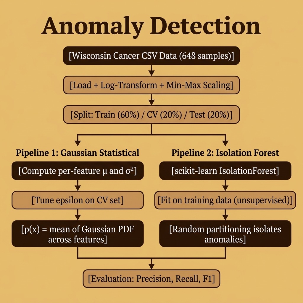
The key insight is that we can build a model of what “normal” looks like and then flag anything that doesn’t fit. This chapter implements two complementary approaches:
- Gaussian Statistical Detector — a from-scratch implementation that models each feature with a Gaussian distribution and uses a tunable probability threshold.
- Isolation Forest — the current industry-standard tree-based algorithm from scikit-learn that requires no labeled data at all.
By comparing both approaches on the same dataset, we will see the tradeoffs between supervised tuning and fully unsupervised detection.
The examples for this chapter are in the directory source-code/anomaly_detection. The project is a modern uv-managed Python package (with pyrefly strict typing, ruff formatting, beartype/typeguard runtime type enforcement, and Claude Code hooks). From the project directory, one command syncs the environment and installs all runtime and dev dependencies (numpy, matplotlib, scikit-learn, pandas, pytest, hypothesis, etc.):
1 uv sync
The justfile provides the developer workflow: just check runs format-check + lint + typecheck + tests, just run runs the Wisconsin example, and just test runs the unit and property-based tests. See the project README.md for the full setup guide.
The Wisconsin Breast Cancer Dataset
We reuse the Wisconsin Diagnostic Breast Cancer dataset from earlier chapters, this time treating malignant samples as anomalies rather than a classification target. The dataset contains 648 samples with 9 features measuring cell characteristics (clump thickness, uniformity of cell size and shape, marginal adhesion, etc.) and a class label: 2 for benign, 4 for malignant.
Roughly 35% of samples are malignant — a higher anomaly rate than most real-world problems, but useful for demonstrating the techniques with enough anomalies to evaluate precision and recall meaningfully.
Data Preprocessing
Good anomaly detection requires careful preprocessing. Many statistical detectors assume features follow an approximately Gaussian (bell-curve) distribution, so we apply a log-transform followed by per-row min–max scaling to push the data closer to that assumption:
 1 raw = np.genfromtxt(DATA_PATH, delimiter=",")
 2 X_raw = raw[:, :9] * 0.1           # scale to [0, 1]
 3
 4 # log-transform to approximate Gaussian shape
 5 X_log = np.log(X_raw + 1.2)
 6 row_min = X_log.min(axis=1, keepdims=True)
 7 row_max = X_log.max(axis=1, keepdims=True)
 8 X = (X_log - row_min) / (row_max - row_min + 1e-10)
 9
10 # Target: map class 2 → 0 (normal), class 4 → 1 (anomaly)
11 y = ((raw[:, 9] - 2) * 0.5).astype(int)
We then split the data three ways — 60% training, 20% cross-validation, 20% test. Crucially, the training set is built from mostly normal (benign) examples, with only about 10% anomalies allowed through. This mimics the real-world scenario where we train on data that is overwhelmingly normal:
 1 # Training set: keep mostly normal (benign) examples,
 2 # allow ~10% anomalies through (matches Java logic)
 3 normal_mask = y[train_idx] == 0
 4 anomaly_mask = y[train_idx] == 1
 5 keep_anomaly = rng.random(anomaly_mask.sum()) < 0.1
 6 keep_idx = np.concatenate([
 7     train_idx[normal_mask],
 8     train_idx[anomaly_mask][keep_anomaly],
 9 ])
10 X_train = X[keep_idx]
The script also generates a 3×3 grid of per-feature histograms colour-coded by class, saved to histograms.png. Examining these distributions is always a good first step — features where the normal and anomaly distributions overlap heavily will be harder for any detector to leverage.
Approach 1: Gaussian Statistical Detector
The Gaussian approach is mathematically elegant and gives deep insight into why anomaly detection works. The idea comes from Andrew Ng’s machine learning course and is a staple of introductory ML curricula.
The Algorithm
For each feature, we compute the mean (μ) and variance (σ²) from the training data. Given a new observation x, we compute the probability of each feature under its Gaussian distribution and average the results:
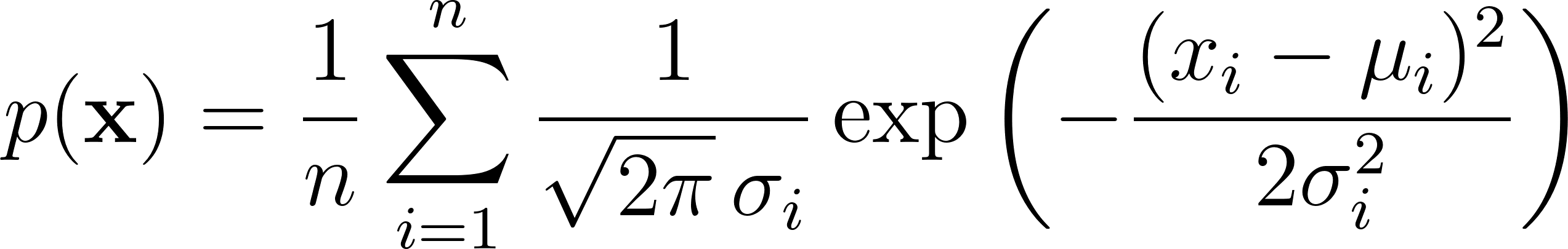
If this aggregate probability falls below a threshold epsilon (ε), the observation is flagged as an anomaly.
Implementation
The GaussianAnomalyDetector class in src/anomaly_detection/detectors.py implements this in about 50 lines of Python:
 1 class GaussianAnomalyDetector:
 2
 3     def __init__(self):
 4         self.mu = None
 5         self.sigma_sq = None
 6         self.epsilon = 0.02
 7
 8     def fit(self, X_train, y_cv=None, X_cv=None):
 9         self.mu = X_train.mean(axis=0)
10         self._fit_sigma(X_train)
11         if X_cv is not None and y_cv is not None:
12             self._tune_epsilon(X_cv, y_cv)
13
14     def _fit_sigma(self, X):
15         self.sigma_sq = (
16             np.sum((X - self.mu) ** 2, axis=0)
17             / X.shape[0]
18         )
19         self.sigma_sq = np.maximum(self.sigma_sq, 1e-10)
20
21     def _probability(self, X):
22         exponent = (
23             -((X - self.mu) ** 2) / (2.0 * self.sigma_sq)
24         )
25         per_feature = (
26             1.0 / (SQRT_2_PI * np.sqrt(self.sigma_sq))
27         ) * np.exp(exponent)
28         return per_feature.mean(axis=1)
29
30     def predict(self, X):
31         return self._probability(X) < self.epsilon
A few things to note:
- The variance is computed as the mean of squared deviations from the mean — the standard formula for population variance.
- We guard against zero variance with
np.maximum(self.sigma_sq, 1e-10)to avoid division by zero in features with constant values. - The
predictmethod returnsTruefor anomalies — observations whose probability falls below epsilon.
Tuning Epsilon
The threshold ε is a hyperparameter that controls the sensitivity of the detector. Too low, and anomalies slip through (low recall). Too high, and normal observations get flagged (low precision).
We tune epsilon on the cross-validation set by sweeping through a range of candidate values and selecting the one that minimises classification errors:
1 def _tune_epsilon(self, X_cv, y_cv):
2     best_err, best_eps = 1e10, self.epsilon
3     for i in range(200):
4         eps = 0.001 + 0.005 * i
5         preds = self._probability(X_cv) < eps
6         err = np.sum(preds != y_cv)
7         if err <= best_err:
8             best_err, best_eps = err, eps
9     self.epsilon = best_eps
Note the <= comparison: when multiple epsilon values produce the same error count, we prefer the highest one. This gives a more generous threshold that is less likely to overfit to the cross-validation set.
Approach 2: Isolation Forest
Isolation Forest, introduced by Fei Tony Liu, Kai Ming Ting, and Zhi-Hua Zhou in 2008, is the industry-standard baseline for anomaly detection on tabular data. The core idea is beautifully simple: anomalies are easier to isolate than normal points.
How It Works
The algorithm builds an ensemble of random trees (similar to Random Forest, but without labels). Each tree recursively partitions the data by choosing a random feature and a random split point. Normal observations, which are surrounded by similar points, require many splits to isolate. Anomalies, which are few and different, get isolated in just a few splits.
The anomaly score is based on the average path length from the root to the leaf across all trees. Shorter paths mean the observation was easy to isolate — hence, more anomalous.
Implementation
Because scikit-learn provides a high-quality implementation, our wrapper is just a thin adapter that matches the interface of the Gaussian detector:
 1 class IsolationForestDetector:
 2
 3     def __init__(self, contamination=0.1, n_estimators=200,
 4                  random_state=42):
 5         self.model = IsolationForest(
 6             contamination=contamination,
 7             n_estimators=n_estimators,
 8             random_state=random_state,
 9         )
10
11     def fit(self, X_train, y_cv=None, X_cv=None):
12         self.model.fit(X_train)
13
14     def predict(self, X):
15         return self.model.predict(X) == -1
The key hyperparameter is contamination — the expected proportion of anomalies in the training data. Setting this correctly is critical: too low and the model misses anomalies; too high and it over-flags normal data. In our example we set it to 0.35 to match the dataset’s actual anomaly rate.
Unlike the Gaussian detector, Isolation Forest is fully unsupervised — it does not use the cross-validation labels at all. This is both its strength (works without any labels) and its weakness (cannot tune a decision boundary to match known anomaly patterns).
Running the Example
Running the complete example (either just run or the underlying uv run invocation):
 1 $ just run
 2 uv run python -m anomaly_detection.wisconsin
 3 Training examples  : 264
 4 Cross-val examples : 129
 5 Test examples      : 131
 6
 7 Histograms saved to histograms.png
 8   Gaussian detector — best epsilon = 0.9960  (CV errors: 16)
 9
10 ──────────────────────────────────────────────────
11   Gaussian Statistical Detector
12 ──────────────────────────────────────────────────
13   Precision : 0.9024
14   Recall    : 0.8043
15   F1        : 0.8506
16
17               precision    recall  f1-score   support
18
19       normal       0.90      0.95      0.93        85
20      anomaly       0.90      0.80      0.85        46
21
22     accuracy                           0.90       131
23    macro avg       0.90      0.88      0.89       131
24   weighted avg       0.90      0.90      0.90       131
25
26
27 ──────────────────────────────────────────────────
28   Isolation Forest Detector
29 ──────────────────────────────────────────────────
30   Precision : 0.5897
31   Recall    : 1.0000
32   F1        : 0.7419
33
34               precision    recall  f1-score   support
35
36       normal       1.00      0.62      0.77        85
37      anomaly       0.59      1.00      0.74        46
38
39     accuracy                           0.76       131
40    macro avg       0.79      0.81      0.76       131
41   weighted avg       0.86      0.76      0.76       131
Interpreting the Results
The results reveal an important lesson about the tradeoff between supervised and unsupervised approaches:
Gaussian Detector (F1 = 0.85): Because it uses cross-validation labels to tune epsilon, it achieves excellent balance — 90% precision with 80% recall. It correctly classifies 90% of all test samples.
Isolation Forest (F1 = 0.74): It catches every anomaly (100% recall) but at the cost of many false positives (59% precision). It flags 38% of normal samples as anomalous. This is a common characteristic of unsupervised detectors — they err on the side of caution.
The takeaway: when you have even a small set of labeled anomalies for tuning, a simpler statistical model can outperform a more sophisticated unsupervised one. In practice, many production systems use a hybrid approach — an unsupervised detector for initial screening, followed by a tuned model (or human review) for the final decision.
Evaluation Metrics for Anomaly Detection
Standard accuracy is misleading for anomaly detection because the classes are imbalanced. If 95% of data is normal, a model that always predicts “normal” achieves 95% accuracy while catching zero anomalies. Instead, focus on:
- Precision: Of the observations flagged as anomalies, how many actually are? High precision means few false alarms.
- Recall: Of all true anomalies, how many did we catch? High recall means few missed anomalies.
- F1 Score: The harmonic mean of precision and recall — a single number that balances both concerns.
The right balance depends on your domain. In fraud detection, missing a fraud (low recall) is costly, so you tolerate more false positives. In manufacturing, false alarms that shut down a production line (low precision) are costly, so you set a higher threshold.
Anomaly Detection Wrap-up
In this chapter we implemented two complementary approaches to anomaly detection:
- The Gaussian statistical detector gives us mathematical transparency: we can inspect the learned μ and σ² values per feature and understand exactly why an observation was flagged. The epsilon threshold provides a single, interpretable knob for controlling sensitivity.
- The Isolation Forest requires no labels and scales well to high-dimensional data. It is the recommended starting point for any new anomaly detection project where labeled anomalies are unavailable.
Both approaches are widely used in practice, and understanding their tradeoffs — supervised tuning vs. unsupervised convenience, interpretability vs. scalability — is essential for any practitioner working with anomaly detection problems.
Optional Practice Problems
Here are some optional practice problems to help you deepen your understanding of anomaly detection and extend the code implemented in this chapter.
Problem 1 (Easy): Independent Gaussian Log-Likelihood
The current implementation of the GaussianAnomalyDetector computes the arithmetic mean of the individual feature probabilities to determine the overall probability of a sample:
1 return per_feature.mean(axis=1)
If we assume that the features are conditionally independent given the class, the joint probability of a sample is the product of its feature probabilities:
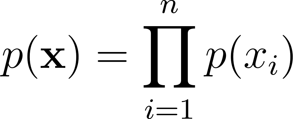
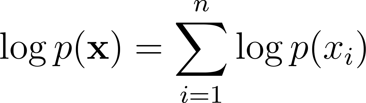
Because multiplying small probabilities leads to numerical underflow, we typically compute the sum of log-probabilities instead:
Task:
- Modify the
_probabilitymethod of GaussianAnomalyDetector to compute the joint log-probability of each sample. (Hint: compute the natural logarithm of individual feature probability densities, sum them across axis 1, and return this log-probability). - Update the
_tune_epsilonandpredictmethods accordingly. Note that since log-probabilities are negative numbers,epsilonwill also be negative, and a sample is an anomaly when its log-probability is lower (more negative) thanepsilon. You will need to adjust the range of candidate thresholds swept in_tune_epsilon. - Tune
epsilonon the cross-validation set and evaluate the new log-likelihood detector on the test set. - Compare the resulting Precision, Recall, and F1 scores with those of the original arithmetic-mean implementation.
Problem 2 (Medium): Semi-Supervised Hyperparameter Tuning for Isolation Forest
Currently, our IsolationForestDetector wrapper is fully unsupervised and uses a hardcoded contamination=0.35 hyperparameter:
1 iforest = IsolationForestDetector(contamination=0.35)
In real-world settings, we often have a small labeled dataset (e.g., our cross-validation set) that we can use to tune hyperparameters, even if the model itself is trained in an unsupervised manner on the training set.
Task:
-
Implement a grid search within
fitthat sweeps over a range of hyperparameters when validation data is provided:contamination: from0.05to0.50in steps of0.05n_estimators:[50, 100, 200, 300]
- For each combination, fit the
IsolationForestmodel onX_train, predict onX_cv, and calculate the validation F1 score. - Store the best-performing hyperparameters and fit the final model using them.
- Integrate this tuning step in wisconsin_anomaly.py, evaluate the optimized model on the test set, and compare the results to the default model. How much did tuning improve the Precision and F1 score?
Problem 3 (Hard): Density-based Detection with Local Outlier Factor (LOF) and PCA
While Isolation Forest isolates anomalies using random partitioning, distance- or density-based methods like Local Outlier Factor (LOF) identify anomalies by comparing the local density of a point to that of its neighbors. In high-dimensional spaces, these density metrics can degrade due to the “curse of dimensionality.”
Task:
- Implement a new class
LOFDetectorin anomaly_detection.py wrapping scikit-learn’sLocalOutlierFactor. Setnovelty=Truein the constructor so you can callfiton training data andpredict/scoreon test data. - Write a Python script that applies Principal Component Analysis (PCA) to reduce the 9-dimensional cancer dataset to 2 dimensions.
-
Train all three detectors (GaussianAnomalyDetector, IsolationForestDetector, and your new
LOFDetector) on:- The original 9-dimensional space.
- The 2-dimensional PCA space.
- Evaluate and compare the Precision, Recall, and F1 scores for all configurations on the test set.
-
Using
matplotlib, plot the 2D PCA-reduced test set. Create subplots showing:- The true class labels (normal vs. anomaly).
- The predictions of each detector (correctly identified normal points, true positives, false positives, and false negatives).
- Analyze which patterns each detector struggled with or excelled at resolving.