Benchmarking Model Inference Speeds

When working with local large language models through Ollama, one of the most practical questions you face is: which model should I use for a given task? Model selection is rarely about picking the “best” model in the abstract because it’s about finding the best trade-off between response quality, inference speed, and the memory footprint your hardware can support. A model that produces beautiful prose is of limited use if it takes two minutes to answer a simple question on your laptop.

This chapter provides a hands-on utility for measuring inference speed across different models on your own hardware. The examples for this chapter are in the directory benchmarking_model_inference_speeds.

Dear reader, this chapter provides suggestions and example code for comparing inference speeds of models running on Ollama. In my personal research I prefer using local models for appropriate use cases and I run open models on inference providers like, for example, FireWorks.ai. You can use the ideas presented here to also evaluate inference speed on commercial APIs.

Most published benchmark numbers (tokens per second, time-to-first-token, etc.) are measured on high-end GPUs that bear little resemblance to the MacBook or Linux workstation on your desk. The only reliable benchmark is one you run yourself.

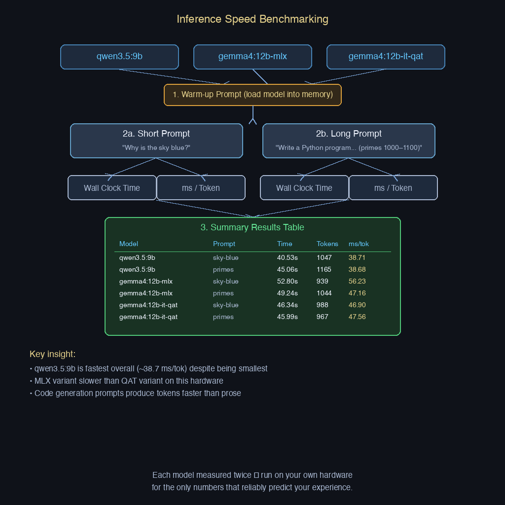
Our approach is deliberately simple:

1. Warm up each model with a short prompt to ensure it is loaded into GPU/system memory.
2. Time wall-clock inference on two qualitatively different prompts: a short factual question and a longer code-generation task.
3. Report both total elapsed time and milliseconds per output token.

Wall-clock time captures the full user experience: model loading delays (mitigated by the warm-up), prompt processing, and token generation. The per-token metric normalizes for the fact that different models may produce outputs of different lengths.

The following listing shows the full inference_speed_tests.py utility:

Model list. The MODELS constant at the top of the file defines the three models we are benchmarking. You can edit this list to add or remove models that you have pulled locally with ollama pull <model>.

Warm-up. The warmup function sends a trivial classification prompt (“identify which numbers are even”) to the model using Ollama’s chat API in non-streaming mode. The warm-up serves two purposes: it forces Ollama to load the model weights into memory, and it populates Ollama’s internal KV cache with the prompt prefix. Without a warm-up, the first timed benchmark would include model-loading overhead, skewing the results.

Benchmark function. The benchmark function streams the model’s response and times the operation from the moment the first chunk is requested until the final chunk arrives. Streaming is used so we can measure wall-clock time that includes time-to-first-token which is the latency the user actually experiences while waiting for the response to start appearing.

The function counts tokens from each chunk, but then overrides that count with eval_count from the final chunk. The Ollama streaming API includes eval_count only in the last chunk of the response, and it is the definitive count of generated tokens. Using it ensures an accurate tokens-per-second calculation even if individual chunks contain partial tokens.

Result formatting. The format_row helper computes milliseconds per token and returns a formatted table row string. The main function orchestrates the full loop: for each model, warm up, run both benchmarks, and accumulate results. A summary table is printed at the end using box-drawing characters.

Running the script on a MacBook Pro with an M2 Pro chip and 32 GB of memory produces something like the following:

Several patterns emerge from these numbers:

The 9B parameter model (qwen3.5:9b) is the fastest on both prompts, generating tokens at roughly 39 ms each. This is expected because fewer parameters means fewer matrix multiplications per token. Despite the smaller size, it produced the longest responses (1047 and 1165 tokens), suggesting it was more verbose in its explanations.

The MLX-optimized Gemma variant (gemma4:12b-mlx) is noticeably slower than the QAT variant on both prompts. MLX is Apple’s machine learning framework optimized for Apple Silicon, and while it can sometimes offer other advantages, on this hardware it did not translate to faster token generation for this particular model.

Both Gemma variants show a per-token speed gap between prompts. The sky-blue prompt ran at 56.23 ms/token on the MLX variant but the primes prompt ran at 47.16 ms/token: about 16% faster. This is counterintuitive since the primes prompt produced more tokens. The likely explanation is that code generation involves more predictable token sequences (syntax keywords, common variable names) that the model’s output head can sample faster than the more varied vocabulary of prose explanation.

The QAT variant shows near-identical per-token speed across both prompts (46.90 vs 47.56 ms/token), suggesting it has more consistent generation behavior than the MLX variant.

Your results will differ. The numbers depend on your specific hardware (CPU, GPU, unified memory bandwidth), the current system load, and even whether the model weights fit entirely in GPU memory or spill over into slower system RAM. Run the benchmark on your own machine and trust your own numbers.

A few important things this utility does not capture:

Response quality. A fast model that gives wrong answers is worse than a slow model that is accurate. Inference speed is one axis of a multi-dimensional trade-off. After running the benchmarks, review the actual responses to see if the faster model’s output is acceptable for your use case.

Prompt processing time. By streaming the response, the timer starts when the first token is requested and stops when the last token arrives. This includes the prompt evaluation phase (the model’s forward pass over the input tokens) and the generation phase. Ollama’s API also returns prompt_eval_duration in nanoseconds, which you could extract to separate prompt processing from token generation, as we demonstrated in the Prompt Caching chapter.

Memory usage. A 12B parameter model at 4-bit quantization occupies roughly 7–8 GB of memory. If your system has 16 GB of RAM and you have other applications open, the model may not fit entirely in GPU memory, causing slower inference as data moves between system RAM and the GPU. The benchmark will reveal the speed impact, but it will not tell you why it is slower.

Batch throughput. This benchmark sends one request at a time. Production systems often batch multiple requests to saturate the GPU’s compute units. Single-request latency and multi-request throughput are different metrics.

The script is designed to be easy to modify:

Adding models. Edit the MODELS list at the top of the file. Any model pulled locally with ollama pull can be added.

Changing the prompts. Edit PROMPT_SKY and PROMPT_PRIMES to test different types of tasks such as translation, summarization, classification, etc. For a fair comparison, use prompts that are likely to produce outputs of similar length across models, or always report the per-token metric.

Adding more prompts. Extend the for label, prompt in [...] loop in main() with additional (label, prompt) pairs.

Exporting results. Replace the print statements with CSV or JSON output for further analysis in a spreadsheet or plotting tool.

Benchmarking inference speed on your own hardware is one of the highest-value activities you can perform when starting a new Ollama-based project. The ten minutes it takes to run these tests will pay for themselves many times over by preventing you from committing to a model that is too slow for interactive use.

The utility in this chapter gives you a baseline. From here, you can experiment with quantization levels (e.g., comparing qwen3.5:9b-q4_K_M vs qwen3.5:9b-q8_0), context window sizes, and the num_gpu parameter to see how they affect inference speed on your specific machine.

1. Quantization-Level Comparison. Pull two different quantization levels of the same base model, for example qwen3.5:9b-q4_K_M and qwen3.5:9b-q8_0. Add both to the MODELS list and run the benchmark. Compare the per-token speeds. Does the higher-precision model produce noticeably better responses, or is the speed difference the main trade-off? Write a short paragraph summarizing your findings.

2. Context Window Stress Test. Modify the script to add a third prompt category: a long prompt that includes several pages of text (use Path("../data/economics.txt").read_text() from the Prompt Caching chapter) followed by a short question. Measure both inference time and prompt evaluation time (prompt_eval_duration from the response). Compare how different models handle long-context scenarios.

3. Time-to-First-Token Measurement. The current benchmark measures total wall-clock time. Modify the benchmark function to also record the time when the first non-empty content chunk arrives. Print both time-to-first-token and total generation time. Which model has the lowest latency before the user sees the first word?

4. Multi-Run Averaging. LLM inference is stochastic and system load varies. Modify main() to run each benchmark three times and report the average and standard deviation of wall-clock time and ms/token. Does the ranking of models remain consistent across runs, or does variability change the ordering?

5. Memory Usage Monitoring. On macOS, use the psutil library to sample memory usage (psutil.virtual_memory().used) before and after loading each model. Add a “Memory (GB)” column to the summary table. Do larger models always use proportionally more memory, or do some model families compress more efficiently?