Single Temperature Measurement

This project will measure temperature using a single DS18B20 sensor. This project will use the waterproof version of the sensor since it has more potential practical applications.

Measure

Hardware required

• DS18B20 sensor (the waterproof version)
• 10k Ohm resister
• Jumper cables
• Cobbler Board
• Ribbon cable

Connect

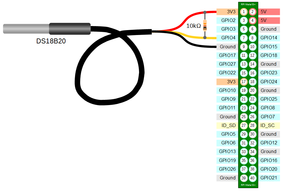
The DS18B20 sensor needs to be connected with the black wire to ground, the red wire to the 3V3 pin and the blue or yellow (some are blue and some are yellow) wire to the GPIO4 pin. A resistor between the value of 4.7k Ohms to 10k Ohms needs to be connected between the 3V3 and GPIO4 pins to act as a ‘pull-up’ resistor.

The Raspbian Operating System image that we are using only supports GPIO4 as a 1-Wire pin, so we need to ensure that this is the pin that we use for connecting our temperature sensor.

The following diagram is a simplified view of the connection.

To connect the sensor practically can be achieved in a number of ways. You could use a Pi Cobbler break out connector mounted on a bread board connected to the GPIO pins.

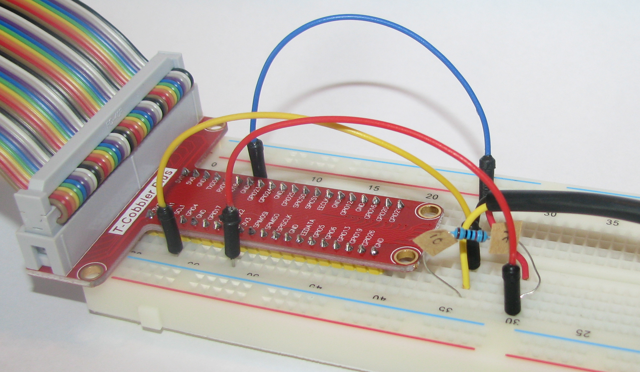
Or we could build a minimal configuration that will plug directly onto the appropriate GPIO pins.

Test

Because the Raspberry Pi acts like an embedded platform rather than a regular PC, it doesn’t have a BIOS (Basic Input Output System) that goes through the various pieces of hardware when the Pi boots up and configures everything. Instead it has an optional text file named config.txt. This can be found in the /boot directory. To enable the Pi to use the GPIO pin to communicate with our temperature sensor we need to tell it to configure itself with the w1-gpio Onewire interface module.

We can do this by editing the /boot/config.txt file using…

…and adding in the line…

dtoverlay=w1-gpio

…at the end of the file

After making this change we need to reboot our Pi to let the changes take effect;

From the terminal as the ‘pi’ user run the command;

modprobe w1-gpio registers the new sensor connected to GPIO4 so that now the Raspberry Pi knows that there is a 1-Wire device connected to the GPIO connector (For more information on the modprobe command check out the Glossary).

Then run the command;

modprobe w1-therm tells the Raspberry Pi to add the ability to measure temperature on the 1-Wire system.

Then we change into the /sys/bus/w1/devices directory and list the contents using the following commands;

(For more information on the cd command check out the Glossary here. Or to find out more about the ls command go here)

This should list out the contents of the /sys/bus/w1/devices which should include a directory starting 28-. The portion of the name following the 28- is the unique serial number of the sensor.

We then change into that unique directory;

We are then going to view the ‘w1_slave’ file with the cat command using;

The output should look something like the following;

73 01 4b 46 7f ff 0d 10 41 : crc=41 YES
73 01 4b 46 7f ff 0d 10 41 t=23187

At the end of the first line we see a YES for a successful CRC check (CRC stands for Cyclic Redundancy Check, a good sign that things are going well). If we get a response like NO or FALSE or ERROR, it will be an indication that there is some kind of problem that needs addressing. Check the circuit connections and start troubleshooting.

At the end of the second line we can now find the current temperature. The t=23187 is an indication that the temperature is 23.187 degrees Celsius (we need to divide the reported value by 1000).

Record

To record this data we will use a Python program that checks the sensor every minute and writes the temperature (with a time stamp) into our MySQL database.

Database preparation

First we will set up our database table that will store our data.

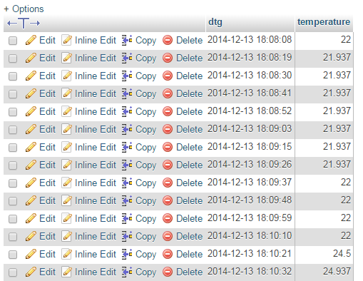
Using the phpMyAdmin web interface that we set up, log on using the administrator (root) account and select the ‘measurements’ database that we created as part of the initial set-up.

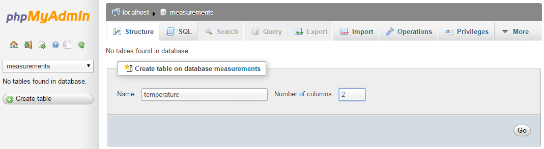
Enter in the name of the table and the number of columns that we are going to use for our measured values. In the screenshot above we can see that the name of the table is ‘temperature’ (how imaginative) and the number of columns is ‘2’.

We will use two columns so that we can store a temperature reading and the time it was recorded.

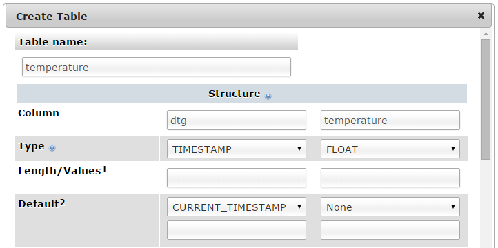
Once we click on ‘Go’ we are presented with a list of options to configure our table’s columns. Don’t be intimidated by the number of options that are presented, we are going to keep the process as simple as practical.

For the first column we can enter the name of the ‘Column’ as ‘dtg’ (short for date time group) the ‘Type’ as ‘TIMESTAMP’ and the ‘Default’ value as ‘CURRENT_TIMESTAMP’. For the second column we will enter the name ‘temperature’ and the ‘Type’ is ‘FLOAT’ (we won’t use a default value).

Scroll down a little and click on the ‘Save’ button and we’re done.

Record the temperature values

The following code (which is based on the code that is part of the great temperature sensing tutorial on Adafruit) is a Python script which allows us to check the temperature reading from the sensor approximately every 10 seconds and write it to our database.

The full code can be found in the code samples bundled with this book (s_temp.py).

#!/usr/bin/python
# -*- coding: utf-8 -*-

import os
import glob
import time
import MySQLdb as mdb

os.system('modprobe w1-gpio')
os.system('modprobe w1-therm')

base_dir = '/sys/bus/w1/devices/'
device_folder = glob.glob(base_dir + '28*')[0]
device_file = device_folder + '/w1_slave'

def read_temp_raw():
    f = open(device_file, 'r')
    lines = f.readlines()
    f.close()
    return lines

def read_temp():
    lines = read_temp_raw()
    while lines[0].strip()[-3:] != 'YES':
        time.sleep(0.2)
        lines = read_temp_raw()
    equals_pos = lines[1].find('t=')
    if equals_pos != -1:
        temp_string = lines[1][equals_pos+2:]
        temp_c = float(temp_string) / 1000.0
        return temp_c

while True:

    try:
        pi_temp = read_temp()
        con = mdb.connect('localhost', \
                          'pi_insert', \
                          'xxxxxxxxxx', \
                          'measurements');
        cur = con.cursor()
        cur.execute("""INSERT INTO temperature(temperature) \
                       VALUES(%s)""", (pi_temp))
        con.commit()

    except mdb.Error, e:
        con.rollback()
        print "Error %d: %s" % (e.args[0],e.args[1])
        sys.exit(1)

    finally:
        if con:
            con.close()

	time.sleep(10)

This script can be saved in our home directory (/home/pi) and needs to be run as root (sudo) as follows;

While we won’t see much happening at the command line, if we use our web browser to go to the phpMyAdmin interface and select the ‘measurements’ database and then the ‘temperature’ table we will see a range of temperature measurements and their associated time of reading presented.

Code Explanation

The script starts by importing the modules that it’s going to use for the process of reading and recording the temperature measurements;

import os
import glob
import time
import MySQLdb as mdb

The program then issues the modprobe commands that start the interface to the sensor;

os.system('modprobe w1-gpio')
os.system('modprobe w1-therm')

Then we need to find the file (w1_slave) where the readings are being recorded in much the same way that we did it manually earlier;

base_dir = '/sys/bus/w1/devices/'
device_folder = glob.glob(base_dir + '28*')[0]
device_file = device_folder + '/w1_slave'

We then set the function for reading the temperature in a ‘raw’ form from the w1_slave file using the read_temp_raw function that fetches the two lines of messaging from the interface.

def read_temp_raw():
    f = open(device_file, 'r')
    lines = f.readlines()
    f.close()
    return lines

The read_temp function is then declared which checks for bad messages and keeps reading until it gets a message with ‘YES’ on end of the first line. Then the function returns the value of the temperature in degrees C.

def read_temp():
    lines = read_temp_raw()
    while lines[0].strip()[-3:] != 'YES':
        time.sleep(0.2)
        lines = read_temp_raw()
    equals_pos = lines[1].find('t=')
    if equals_pos != -1:
        temp_string = lines[1][equals_pos+2:]
        temp_c = float(temp_string) / 1000.0
        return temp_c

From here we enter into a while loop to continually read the temperature and insert the value into the MySQL database;

while True:

    try:
        pi_temp = read_temp()
        con = mdb.connect('localhost', \
                          'pi_insert', \
                          'xxxxxxxxxx', \
                          'measurements');
        cur = con.cursor()
        cur.execute("""INSERT INTO temperature(temperature) \
                       VALUES(%s)""", (pi_temp))
        con.commit()

    except mdb.Error, e:
        con.rollback()
        print "Error %d: %s" % (e.args[0],e.args[1])
        sys.exit(1)

    finally:
        if con:
            con.close()

	time.sleep(10)

The while statement takes an expression and executes the loop body while the expression evaluates to (boolean) “true”. True executes the loop body indefinitely. Note that most languages usually have some way of breaking out of the loop early. In the case of Python it’s the break statement (not that it’s used here).

Explore

This section has a working solution for presenting temperature data but is a simple representation and is intended to provide a starting point for the display of data from a measurement process. Our data display techniques will become more advanced as we work out different things to measure. In the mean time, enjoy this simple effort.

The Code

The following code is a PHP file that we can place on our Raspberry Pi’s web server (in the /var/www directory) that will allow us to view all of the results that have been recorded in the temperature directory on a graph;

<?php
$hostname = 'localhost';
$username = 'pi_select';
$password = 'xxxxxxxxxx';

try {
    $dbh = new PDO("mysql:host=$hostname;dbname=measurements", 
                               $username, $password);

    /*** The SQL SELECT statement ***/
    $sth = $dbh->prepare("
       SELECT  `dtg`, `temperature` FROM  `temperature`
    ");
    $sth->execute();

    /* Fetch all of the remaining rows in the result set */
    $result = $sth->fetchAll(PDO::FETCH_ASSOC);

    /*** close the database connection ***/
    $dbh = null;
    
}
catch(PDOException $e)
    {
        echo $e->getMessage();
    }

$json_data = json_encode($result); 
?>

<!DOCTYPE html>
<meta charset="utf-8">
<style> /* set the CSS */

body { font: 12px Arial;}

path {
    stroke: steelblue;
    stroke-width: 2;
    fill: none;
}

.axis path,
.axis line {
    fill: none;
    stroke: grey;
    stroke-width: 1;
    shape-rendering: crispEdges;
}

</style>
<body>

<!-- load the d3.js library -->
<script src="http://d3js.org/d3.v3.min.js"></script>

<script>

// Set the dimensions of the canvas / graph
var margin = {top: 30, right: 20, bottom: 30, left: 50},
    width = 800 - margin.left - margin.right,
    height = 270 - margin.top - margin.bottom;

// Parse the date / time
var parseDate = d3.time.format("%Y-%m-%d %H:%M:%S").parse;

// Set the ranges
var x = d3.time.scale().range([0, width]);
var y = d3.scale.linear().range([height, 0]);

// Define the axes
var xAxis = d3.svg.axis().scale(x)
    .orient("bottom");

var yAxis = d3.svg.axis().scale(y)
    .orient("left").ticks(5);

// Define the line
var valueline = d3.svg.line()
    .x(function(d) { return x(d.dtg); })
    .y(function(d) { return y(d.temperature); });

// Adds the svg canvas
var svg = d3.select("body")
    .append("svg")
        .attr("width", width + margin.left + margin.right)
        .attr("height", height + margin.top + margin.bottom)
    .append("g")
        .attr("transform",
              "translate(" + margin.left + "," + margin.top + ")");

// Get the data
<?php echo "data=".$json_data.";" ?>
data.forEach(function(d) {
	d.dtg = parseDate(d.dtg);
	d.temperature = +d.temperature;
});

// Scale the range of the data
x.domain(d3.extent(data, function(d) { return d.dtg; }));
y.domain([0, d3.max(data, function(d) { return d.temperature; })]);

// Add the valueline path.
svg.append("path")
	.attr("d", valueline(data));

// Add the X Axis
svg.append("g")
	.attr("class", "x axis")
	.attr("transform", "translate(0," + height + ")")
	.call(xAxis);

// Add the Y Axis
svg.append("g")
	.attr("class", "y axis")
	.call(yAxis);

</script>
</body>

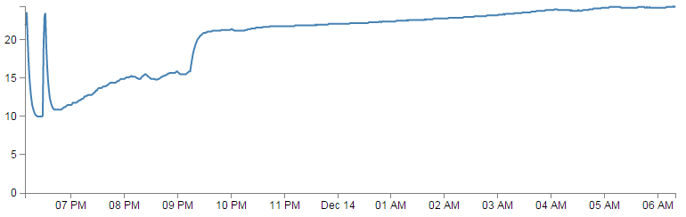
The graph that will look a little like this (except the data will be different of course).

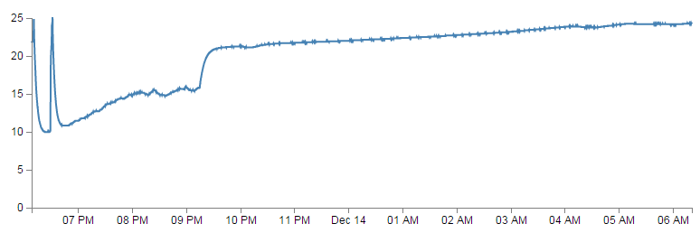
This is a VERY simple graph (i.e, there is no title, labeling of axis or any real embellishment) and as such it has some limitations. For example it will automatically want to display ALL the recorded temperature data in the database. We might initially think that this would be a good thing to do, but in this case there are over 3000 recordings trying to be displayed on a graph that is less than 800 pixels wide. Not only are we not going to see as much detail as could be possible, but the web browser can only cope with a finite amount of data being crammed into it. Eventually it will break.

So as an addendum to the code above we shall look at making a change to our database query to make a slightly more rational selection of data.

Different MySQL Selection Options

Currently our SELECT statement looks like the following;

SELECT  `dtg`, `temperature` FROM  `temperature`

As described earlier, this query is telling the database to SELECT our date/time data (from the dtg column) and the temperature values (from the temperature column) FROM the table temperature. If there are 4 entries in the database, the query will return 4 readings. If there is 400,000 entries in the database, it will return 400,000 readings.

We can limit the number of returned rows to 800 with the query as follows;

SELECT `dtg`, `temperature` FROM  `temperature` LIMIT 0 , 800

This adds in the LIMIT 0,800 specifier which returns 800 rows starting at row ‘0’.

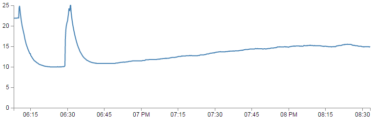
However, this is probably not satisfactory as in the case of the data we have recorded in our Python script, there is only a gap of 10 seconds or so between readings. This restricts us to just over 2 hours worth of recording and the values start when the recording started, so our returned values will never change.

We can improve on this by sorting the returned values and therefore take the most recent ones with the following query;

SELECT `dtg`, `temperature`
FROM `temperature`
ORDER BY `dtg` DESC
LIMIT 0,800

Here we order the returned rows by dtg descending. Which means the most recent date/time value is the one at row ‘0’ and we will capture the most recent two hours worth of readings every time we run the query.

Of course in the case of the data that was in the database, this is a fairly ‘booring’ set with little variation.

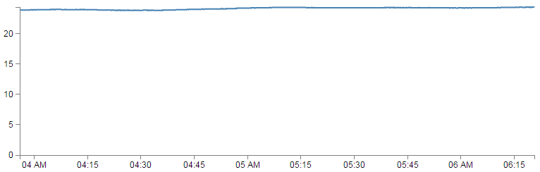
We now have an efficient number of data points being returned to the web browser to graph, but we only see two hours worth of data. It could be argued that the fidelity of reading every 10 seconds is a little high, and if we were to return values for every minute that would be adequate. As an interesting exercise we can return that type of information using our current data set by using a slightly more sophisticated MySQL query;

SELECT
ROUND(AVG(`temperature`),1) AS temperature,
TIMESTAMP(LEFT(`dtg`,16)) AS dtg
FROM `temperature`
GROUP BY LEFT(`dtg`,16)
ORDER BY `dtg` DESC
LIMIT 0,800

Here we are telling MySQL to average our temperature readings (AVG('temperature')) then round the number to 1 decimal place (ROUND(AVG('temperature'),1)) and label the column as ‘temperature’ (AS temperature). At the same time we take the left-most 16 characters of our dtg value (LEFT(dtg,16)) and then convert them back into a TIMESTAMP value (TIMESTAMP(LEFT('dtg',16))). This quirk allows us to eliminate the seconds from our ‘dtg’ values and replace it with ‘00’. We then label the column as ‘dtg’ (AS dtg ).

Now comes the interesting part. We group all the rows that have the same left-most 16 characters (in other words any dtg value that has the same year, month, day, hours and minutes). This has no effect on the dtg values of course, but the temperature values for all the rows with identical dtg’s get mashed together. And in this case we have already told MySQL that we want to average those values out with our earlier ROUND(AVG('temperature'),1) statement.

If we consider the resulting graph, it looks remarkably similar to our original one that included over 3000 points;

The end result has been a ‘smoothing’ of sorts. I can’t claim that it is any better or worse, but it certainly represents the way the temperature varied and does so in a way that won’t break the browser.