Basic GPIO Input Sensors

This project will use a Hall effect sensor to measure a change in a magnetic field and use that change to trigger the recording of a reading to our database. This type of sensor outputs a logical ‘high’ (1) when triggered and as such we can use the same set-up on our Raspberry Pi for a range of sensors.

The practical application that we will examine is to determine when a cat flap has been opened and using the times that this occurs we will build up a visualization of the pattern of activity that the cat exhibits as it goes in and out the cat flap.

For this project we will use a Hall effect sensor combined with circuitry that allows the device to act as a switch. In particular we will use the pre-built sensor ‘KY003’ which incorporates a series 3144 integrated circuit that contains the hall effect sensor proper (and some supporting circuitry). When the sensor is exposed to a high density magnetic field the circuit will produce a logic ‘high’ output. The ‘KY003’ sensor is widely available at an extremely low cost (approximately $2). Just give the part number a Googling for possible sources.

Measure

Hardware required

• KY003 Hall effect sensor
• 3 x Jumper cables
• A magnet (small Rare Earth type would be ideal)

The KY003 Hall Effect Sensor

The KY003 Hall effect sensor has three connections that we will need to connect to a 5V supply, a ‘Ground’ and a GPIO pin to read the signal from the sensor.

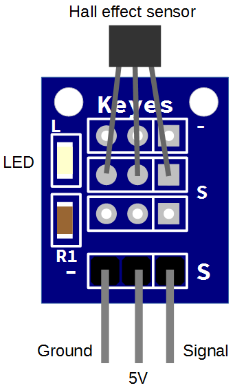
It also incorporates a surface mounted LED that will illuminate when the sensor detects the presence of a magnetic field and is triggered.

Connect

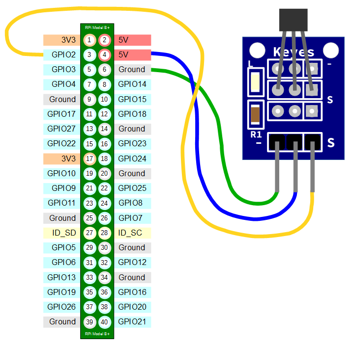
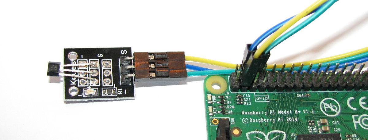
The KY003 sensor should be connected with ground pin to a ground connector, the 5V pin to a 5V connector and the signal pin to a GPIO pin on the on the Raspberry Pi’s connector block. In the connection diagram below the ground is connected to pin 6, the 5V is connected to pin 4 and the signal is connected to pin 3 (GPIO 2)

The following diagram is a simplified view of the connection.

Connecting the sensor practically can be achieved in a number of ways. You could use a Pi Cobbler break out connector mounted on a bread board connected to the GPIO pins. But because the connection is relatively simple we could build a minimal configuration that will plug directly onto the appropriate GPIO pins using header connectors and jumper wire. The image below shows how simple this can be.

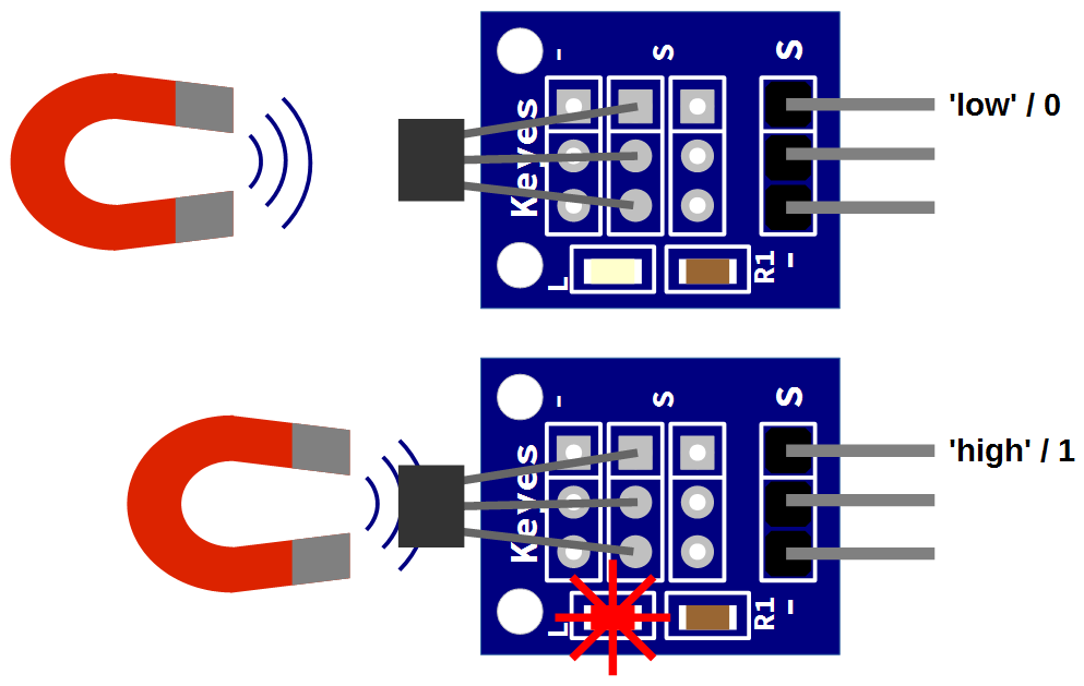
Test

Once correctly connected, the sensor is ready to go. It can be simply tested by bringing a magnet into close proximity with the sensor and the LED should illuminate. When this occurs, we can make the assumption (at this stage) that the sensor is working and has placed ‘high’ or ‘1’ on the signal pin of the sensor and therefore is presenting a ‘high’ or 1’ to GPIO 2 on the Pi.

Record

To record this data we will use a Python program that uses our sensor like a trigger and writes an identifier for the sensor into our MySQL database. At the same time a time stamp will be added automatically. You may be wondering why we’re not recording the value of the sensor (0 or 1) and that’s a valid question. What we are going to use our sensor for is to determine when it has been triggered. For all intents and purposes, we can make the assumption that our sensor represents a device that can be in one of two states. We are going to be interested when it changes state, not when it is steady. In particular we are going to be interested in when it changes from low to high (0 to 1) and therefore represents a ‘rising’ signal.

for this project to work, our Python script has to run continuously and will only write to our database when triggered.

Database preparation

First we will set up our database table that will store our data.

Using the phpMyAdmin web interface that we set up, log on using the administrator (root) account and select the ‘measurements’ database that we created as part of the initial set-up.

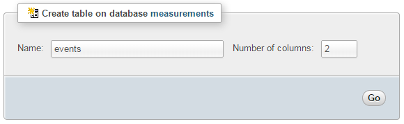
Enter in the name of the table and the number of columns that we are going to use for our measured values. In the screenshot above we can see that the name of the table is ‘events’ and the number of columns is ‘2’.

We will use two columns so that we can store an event name and the time it was recorded.

Once we click on ‘Go’ we are presented with a list of options to configure our table’s columns. Don’t be intimidated by the number of options that are presented, we are going to keep the process as simple as practical.

For the first column we can enter the name of the ‘Column’ as ‘dtg’ (short for date time group) the ‘Type’ as ‘TIMESTAMP’ and the ‘Default’ value as ‘CURRENT_TIMESTAMP’. For the second column we will enter the name ‘event’ and the type is ‘VARCHAR’ with a ‘Length/Values’ of 30.

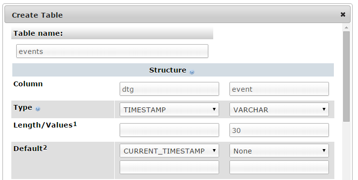
Scroll down a little and click on the ‘Save’ button and we’re done.

Record the events

The following Python code (which is based on the code that is part of the great blog series on FIRSIM) is a script which allows us to check the state of a sensor and write an entry to our database when an event occurs.

The full code can be found in the code samples bundled with this book (events.py).

First a quick shout-out and thanks to the reader ‘salmon’ who kindly suggested a significant change to the original code which changed it from a CPU killing ‘loop of doom’ to a far more well behaved script.

#!/usr/bin/python
# -*- coding: utf-8 -*-

# Import the python libraries
import RPi.GPIO as GPIO
import logging
import MySQLdb as mdb
import time

logging.basicConfig(filename='/home/event_error.log',
  level=logging.DEBUG,
  format='%(asctime)s %(levelname)s %(name)s %(message)s')
logger=logging.getLogger(__name__)

# Function called when GPIO.RISING
def storeFunction(channel):
  print("Signal detected")
  
  con = mdb.connect('localhost', \
                    'pi_insert', \
                    'xxxxxxxxxx', \
                    'measurements');
  
  try:
    cur = con.cursor()
    cur.execute("""INSERT INTO events(event) VALUES(%s)""", ('catflap'))
    con.commit()

  except mdb.Error, e:
    logger.error(e)

  finally:
    if con:
      con.close()

print "Sensor event monitoring (CTRL-C to exit)"

# use the BCM GPIO numbering
GPIO.setmode(GPIO.BCM)

# Definie the BCM-PIN number
GPIO_PIR = 2

# Define pin as input with standard high signaal
GPIO.setup(GPIO_PIR, GPIO.IN, pull_up_down = GPIO.PUD_UP)

try:
  # Loop while true = true
  while True :

    # Wait for the trigger then call the function
    GPIO.wait_for_edge(GPIO_PIR, GPIO.RISING)
    storeFunction(2)
    time.sleep(1)

except KeyboardInterrupt:
  # Reset the GPIO settings
  GPIO.cleanup()

This script can be saved in our home directory (/home/pi) and can be run by typing;

The observant amongst you will notice that we need to run the program as the superuser (by invoking sudo before the command to run events.py). This is because the GPIO library requires the accessing of the GPIO pins to be done by the superuser.

Once the command is run the pi will generate a warning to let us know that there is a pull up resister fitted to channel 2. That’s fine. From here if we move our magnet towards and away from the sensor we should see the Signal detected notification appear in the terminal per below.

pi@raspberrypi ~ $ sudo python event.py
Sensor event monitoring (CTRL-C to exit)
event.py:23: RuntimeWarning: A physical pull up resistor is fitted on this ch\
annel!
  GPIO.setup(GPIO_PIR, GPIO.IN, pull_up_down = GPIO.PUD_UP)
Signal detected
Signal detected

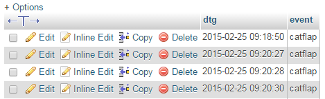
We should then be able to check our MySQL database and see an entry for each time that the sensor triggered.

Code Explanation

The script starts by importing the modules that it’s going to use for the process of reading and recording the measurements;

import RPi.GPIO as GPIO
import logging
import MySQLdb as mdb
import time

Then the code sets up the logging module. We are going to use the basicConfig() function to set up the default handler so that any debug messages are written to the file /home/pi/event_error.log.

logging.basicConfig(filename='/home/event_error.log',
  level=logging.DEBUG,
  format='%(asctime)s %(levelname)s %(name)s %(message)s')
logger=logging.getLogger(__name__)

In the following function where we are getting our readings or writing to the database we write to the log file if there is an error.

Which brings us to our function storeFunction that will write information to our database when called later;

def storeFunction(channel):
  print("Signal detected")
  
  con = mdb.connect('localhost', \
                    'pi_insert', \
                    'xxxxxxxxxx', \
                    'measurements');
  
  try:
    cur = con.cursor()
    cur.execute("""INSERT INTO events(event) VALUES(%s)""", ('catflap'))
    con.commit()
    
  except mdb.Error, e:
    logger.error(e)
    
  finally:    
    if con:    
      con.close()

This is very much a rinse and repeat of the function found in the single temperature project. We configure our connection details, connect and write the name of this particular sensor (‘catflap’) into the database (Remember that when we store an event name into the database the timestamp dtg is added to the record automatically.). We then have some house-keeping code that will log any errors and then close the connection to the database.

The program can then issues the GPIO commands that start the interface to the sensor and get it configured (the code below has been condensed for clarity);

GPIO.setmode(GPIO.BCM)
GPIO_PIR = 2
GPIO.setup(GPIO_PIR, GPIO.IN, pull_up_down = GPIO.PUD_UP)

The GPIO Python module was developed and is maintained by Ben Croston. You can find a wealth of information on its usage at the official wiki site.

GPIO.setmode allows us to tell which convention of numbering the IO pins on the Raspberry Pi we will use when we say that we’re going to read a value off one of them. Observant Pi users will have noticed that the GPIO numbers don’t match the pin numbers. Believe it or not there is a good reason for this and in the words of the good folks from raspberrypi.org;

“While there are good reasons for software engineers to use the BCM numbering system (the GPIO pins can do more than just simple input and output), most beginners find the human readable numbering system more useful. Counting down the pins is simple, and you don’t need a reference or have to remember which is which. Take your pick though; as long as you use the same scheme within a program then all will be well.”

In our case we are using the BCM numbering (GPIO.setmode(GPIO.BCM)).

We then assign the GPIO channel as GPIO 2 to a variable (GPIO_PIR = 2).

Then we configure how we are going to read the GPIO channel with GPIO.setup. We specify the channel with GPIO_PIR, whether the channel will be an input or an output (GPIO.IN) and we configure the Broadcom SCO to use a pull up resistor in software (pull_up_down=GPIO.PUD_UP).

Then the code executes an ‘endless’ loop that asks itself “Is True, True?”. While it is the program essentially pauses while it waits for a signal from the sensor via the GPIO channel.

try:
  # Loop while true = true
  while True :

    # Wait for the trigger then call the function
    GPIO.wait_for_edge(GPIO_PIR, GPIO.RISING)
    storeFunction(2)
    time.sleep(1)

Ultimately True stops being True when the program receives a ‘break’ which can occur with a ‘ctrl-c’ keypress.

In the mean time we’re using wait_for_edge to look for a specific type of event. We specify the channel (GPIO_PIR) we want to look for and the type of change in the channel which is a rising edge (GPIO.RISING) (which signifies a change in state (going from 0 to 1)). When this occurs the program progresses and the storeFunction function is called (which will record the event in the database). Lastly we let the program sleep for 1 second (time.sleep(1)) which reduces the occurrence of false events in the case of the cat flap swinging backwards and forwards when closing. This is the equivalent of ‘debouncing’ a switch.

Finally we use the keyboard interruption of the loop to do some housekeeping and reset our GPOI ports;

except KeyboardInterrupt:
  # Reset the GPIO settings
  GPIO.cleanup()

This results in any of the GPIO ports that have been used in the program being set back to input mode. This occurs because it is safer (for the equipment) to leave the ports as inputs which removes any extraneous voltages.

Start the code automatically at boot

While we can run our script easily from the command line, this is not going to be convenient when we deploy our cat flap activity logger. The alternative is to automatically start the script using rc.local in a similar way that we did with ‘tightvncserver’ in our initial set-up.

We will add the following command into rc.local;

python /home/pi/events.py

This command looks slightly different for the way that we have been running the script so far (sudo python events.py). This is because we do not need to use sudo (since rc.local runs as as the root user already, and we need to specify the full path to the script (/home/pi/events.py) as there is no environment set up in a home directory or similar (i.e. we’re not starting from /home/pi/).

To do this we will edit the rc.local file with the following command;

Add in our lines so that the file looks like the following;

#!/bin/sh -e
#
# rc.local
#
# This script is executed at the end of each multiuser runlevel.
# Make sure that the script will "exit 0" on success or any other
# value on error.
#
# In order to enable or disable this script just change the execution
# bits.
#
# By default this script does nothing.

# Print the IP address
_IP=$(hostname -I) || true
if [ "$_IP" ]; then
  printf "My IP address is %s\n" "$_IP"
fi

# Start tightvncserver
su - pi -c '/usr/bin/tightvncserver :1'

# Start the event monitoring script 
python /home/pi/events.py

exit 0

(We can also add our own comment into the file to let future readers know what’s going on)

That should be it. We should now be able to test that the service starts when the Pi boots by typing in;

Then check our MySQL database to see the events increment as we wave our magnet in front of the Hall effect sensor.

Nice job! We’re measuring and recording a change in a magnetic field!

Explore

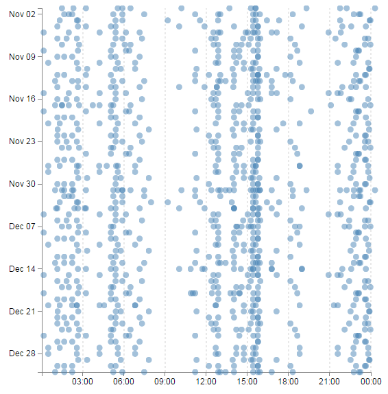
This section has a working solution for presenting data from events,. This is done via a scatter-plot type matrix (hereby referred to as the ‘catter-plot’ as it involves measuring cats going through cat doors) that is slightly different to those that would normally be used. Typically a scatter-plot with use time on the x axis and a value on the Y axis. This example will use the time of day on the X axis, independent of the date and the Y axis will represent the date independent of the time of day. The end result is a scatter-plot where activities that occur on a specific day are seen on a horizontal line and the time of day that these activities occur can form a pattern that the brain can determine fairly easily.

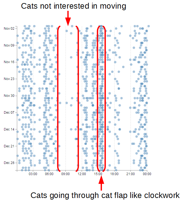
We can easily see that wherever the cats are between approximately 7:30 and 11am they’re not likely to be using the cat door. However, something happens at around 3:30pm and it’s almost certain that they will be coming through the cat flap.

This is a slightly more complex use of JavaScript and d3.js specifically but it is a great platform that demonstrates several powerful techniques for manipulating and presenting data.

It has the potential to be coupled with additional events that could be colour coded and / or they could be sized according to frequency.

The Code

The following code is a PHP file that we can place on our Raspberry Pi’s web server (in the /var/www directory) that will allow us to view all of the results that have been recorded in the temperature directory on a graph;

The full code can be found in the code samples bundled with this book (events.php).

<?php

$hostname = 'localhost';
$username = 'pi_select';
$password = 'xxxxxxxxxx';

try {
    $dbh = new PDO("mysql:host=$hostname;dbname=measurements",
                               $username, $password);

    /*** The SQL SELECT statement ***/
    $sth = $dbh->prepare("
       SELECT dtg
       FROM `events` 
    ");
    $sth->execute();

    /* Fetch all of the remaining rows in the result set */
    $result = $sth->fetchAll(PDO::FETCH_ASSOC);

    /*** close the database connection ***/
    $dbh = null;
}

catch(PDOException $e)
    {
        echo $e->getMessage();
    }

$json_data = json_encode($result);     

?>

<!DOCTYPE html>
<meta charset="utf-8">
<style>

body { font: 12px sans-serif; }

.axis path,
.axis line {
  fill: none;
  stroke: grey;
  shape-rendering: crispEdges;
}

.dot { stroke: none; fill: steelblue; }

.grid .tick { stroke: lightgrey; opacity: 0.7; }
.grid path { stroke-width: 0;}

</style>
<body>
<script src="http://d3js.org/d3.v3.min.js"></script>
<script>

// Get the data
<?php echo "data=".$json_data.";" ?>

// Parse the date / time formats
parseDate = d3.time.format("%Y-%m-%d").parse;
parseTime = d3.time.format("%H:%M:%S").parse;

data.forEach(function(d) {
    dtgSplit = d.dtg.split(" ");     // split on the space
    d.date = parseDate(dtgSplit[0]); // get the date seperatly
    d.time = parseTime(dtgSplit[1]); // get the time separately
});

// Get the number of days in the date range to calculate height
var oneDay = 24*60*60*1000; // hours*minutes*seconds*milliseconds
var dateStart = d3.min(data, function(d) { return d.date; });
var dateFinish = d3.max(data, function(d) { return d.date; });
var numberDays = Math.round(Math.abs((dateStart.getTime() -
                           dateFinish.getTime())/(oneDay)));

var margin = {top: 40, right: 20, bottom: 30, left: 100},
    width = 600 - margin.left - margin.right,
    height = numberDays * 8;

var x = d3.time.scale().range([0, width]);
var y = d3.time.scale().range([0, height]);

var xAxis = d3.svg.axis()
    .scale(x)
    .orient("bottom")
    .ticks(7)
    .tickFormat(d3.time.format("%H:%M"));

var yAxis = d3.svg.axis()
    .scale(y)
    .orient("left")
    .ticks(7,0,0);

var svg = d3.select("body")
    .append("svg")
        .attr("width", width + margin.left + margin.right)
        .attr("height", height + margin.top + margin.bottom)
    .append("g")
        .attr("transform", "translate(" + margin.left + ","
                                        + margin.top + ")");

// State the functions for the grid
function make_x_axis() {
    return d3.svg.axis()
      .scale(x)
      .orient("bottom")
      .ticks(7)
}
        
// Set the domains
x.domain([new Date(1899, 12, 01, 0, 0, 1), 
          new Date(1899, 12, 02, 0, 0, 0)]);
y.domain(d3.extent(data, function(d) { return d.date; }));

// tickSize: Get or set the size of major, minor and end ticks
svg.append("g").classed("grid x_grid", true)
    .attr("transform", "translate(0," + height + ")")
    .style("stroke-dasharray", ("3, 3, 3"))
    .call(make_x_axis()
        .tickSize(-height, 0, 0)
        .tickFormat(""))

// Draw the Axes and the tick labels
svg.append("g")
    .attr("class", "x axis")
    .attr("transform", "translate(0," + height + ")")
    .call(xAxis)
  .selectAll("text")
    .style("text-anchor", "middle");

svg.append("g")
    .attr("class", "y axis")
    .call(yAxis)
  .selectAll("text")
    .style("text-anchor", "end");

// draw the plotted circles
svg.selectAll(".dot")
    .data(data)
  .enter().append("circle")
    .attr("class", "dot")
    .attr("r", 4.5)
    .style("opacity", 0.5)
    .attr("cx", function(d) { return x(d.time); })
    .attr("cy", function(d) { return y(d.date); });    

</script>
</body>

The graph that will look a little like this (except the data will be different of course).

This is a fairly basic graph (i.e, there is no title or labelling of axis).

The code will automatically try to collect as many events as are in the database, so depending on your requirements we may need to vary the query. As some means of compensation it will automatically increase the vertical size of the graph depending on how many days the data spans.

PHP

The PHP block at the start of the code is mostly the same as our example code for our single temperature measurement project. The significant difference however is in the select statement.

       SELECT dtg
       FROM `events` 
       LIMIT 0,900

Here we are only returning a big list of date / time values.

CSS (Styles)

There are a range of styles that are applied to the elements of the graphic.

body { font: 12px sans-serif; }

.axis path,
.axis line {
  fill: none;
  stroke: grey;
  shape-rendering: crispEdges;
}

.dot { stroke: none; fill: steelblue; }

.grid .tick { stroke: lightgrey; opacity: 0.7; }
.grid path { stroke-width: 0;}

We set a default text font and size, some formatting for our axes and grid lines and the colour and type of outline (none) that our dots for our events have.

JavaScript

The code has very similar elements to our single temperature measurement script and comparing both will show us that we are doing similar things in each graph. Interestingly, this code mixes the sequence of some of the ‘blocks’ of code. This is in order to allow the dynamic adjustment of the vertical size of the graph.

The very first thing we do with our JavaScript is to use our old friend PHP to declare our data;

<?php echo "data=".$json_data.";" ?>

Then we declare the two functions we will use to format our time values;

parseDate = d3.time.format("%Y-%m-%d").parse;
parseTime = d3.time.format("%H:%M:%S").parse;

parseDate will format and date values and parseTime will format any time values.

Then we cycle through our data using a forEach statement;

data.forEach(function(d) {
    dtgSplit = d.dtg.split(" ");     // split on the space
    d.date = parseDate(dtgSplit[0]); // get the date seperatly
    d.time = parseTime(dtgSplit[1]); // get the time seperatly
});

In this loop we split our dtg value into date and time portions and then use our parse statements to ensure that they are correctly formatted.

We then do a little bit of date / time maths to work out how many days are between the first day in our range of data and the last day;

var oneDay = 24*60*60*1000; // hours*minutes*seconds*milliseconds
var dateStart = d3.min(data, function(d) { return d.date; });
var dateFinish = d3.max(data, function(d) { return d.date; });
var numberDays = Math.round(Math.abs((dateStart.getTime() -
                           dateFinish.getTime())/(oneDay)));

We set up the size of the graph and the margins (this is where we adjust the height of the graph depending on the number of days);

var margin = {top: 40, right: 20, bottom: 30, left: 100},
    width = 600 - margin.left - margin.right,
    height = numberDays * 8;

The scales and ranges for both axes are both time based in this example;

var x = d3.time.scale().range([0, width]);
var y = d3.time.scale().range([0, height]);

And we set up the x axis and y axis accordingly;

var xAxis = d3.svg.axis()
    .scale(x)
    .orient("bottom")
    .ticks(7)
    .tickFormat(d3.time.format("%H:%M"));

var yAxis = d3.svg.axis()
    .scale(y)
    .orient("left")
    .ticks(7,0,0);

We then create our svg container with the appropriate with and height taking into account the margins;

var svg = d3.select("body")
    .append("svg")
        .attr("width", width + margin.left + margin.right)
        .attr("height", height + margin.top + margin.bottom)
    .append("g")
        .attr("transform", "translate(" + margin.left + ","
                                        + margin.top + ")");

Then we declare a special function that we will use to make our grid;

function make_x_axis() {
    return d3.svg.axis()
      .scale(x)
      .orient("bottom")
      .ticks(7)
}

Essentially we will be creating another x axis with lines that extend the full height of the graph.

Our domains are set in a bit of an unusual way since our time variables have no associated date. Therefore we tell the range to fall over a suitable time range that spans a single day

x.domain([new Date(1899, 12, 01, 0, 0, 1), 
          new Date(1899, 12, 02, 0, 0, 0)]);
y.domain(d3.extent(data, function(d) { return d.date; }));

The y domain can exist as normal although is (unusually) a time scale and not ordinal.

Our grid is added as a separate axis with really tall ticks (tickSize), no text values (tickFormat) and with a dashed line (stroke-dasharray);

svg.append("g").classed("grid x_grid", true)
    .attr("transform", "translate(0," + height + ")")
    .style("stroke-dasharray", ("3, 3, 3"))
    .call(make_x_axis()
        .tickSize(-height, 0, 0)
        .tickFormat(""))

Then we do the mundane adding of the axes and plotting the circles;

Wonderful! And as an added bonus you can also find the file ‘events-tips.php’ in the downloads with the book. This file is much the same as the one we have just explained, but also includes a tool-tip feature that shows the time and date of an individual point when our mouse moves over the top of it.

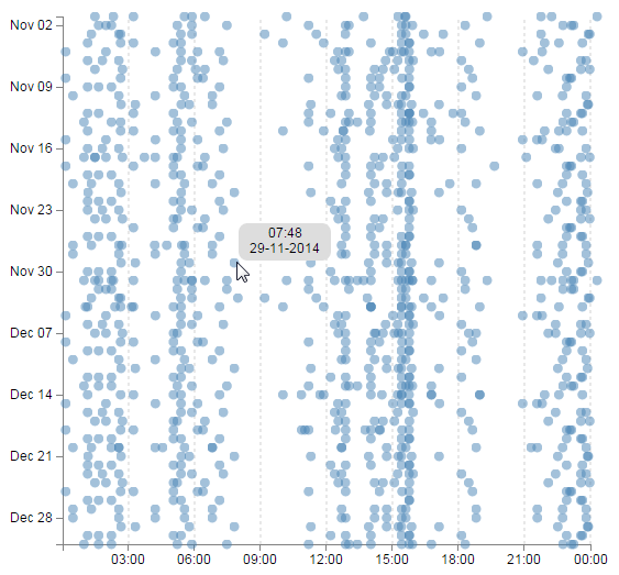
If you want a closer explanation for this piece of code, download a copy of D3 Tips and Tricks for this and a whole swag of other information.