Web Scraping

The term ‘web scraping’ refers to the process of programmatically retrieving data from a web page. There are a wide range of ways that it can be accomplished and there is a degree of responsibility that needs to be taken to do it in a way that doesn’t violate Wheaton’s law.

OK, so what is web scraping?

Web scraping is the act of retrieving some form of information from a web page. The example we will work through is where we want to be able to collect, store and compare the number of readers of the books R Programming for Data Science and The Elements of Data Analytic Style by Messrs Roger Peng and Jeff Leek respectively.

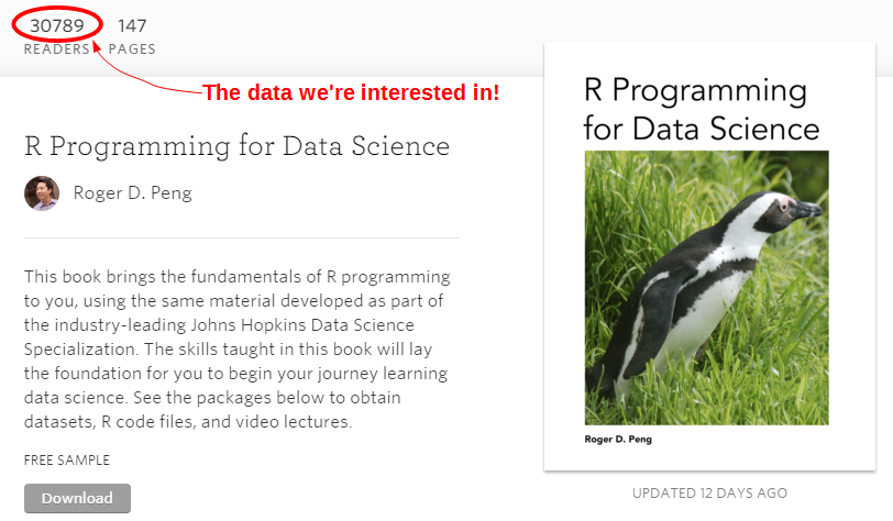
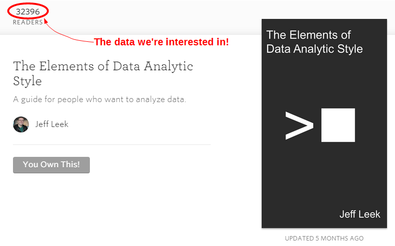
We will check the check the main page of each book every day, store the number of readers in a database and after a period of time we will be able to compare the number or readers that each book gains in a day using a difference chart.

Measure

Hardware required

Only the Raspberry Pi and an internet connection! All the data that we’re going to source will come from the internet.

Software required

The technique that we’ll use to scrape the pages will use the PHP ‘curl’ library. cURL is a command line tool for transferring data with a URL syntax, such as (but not limited to) FTP, HTTP, HTTPS, POP3, SFTP and SMTP. The integration of cURL into PHP give us a programmatic way to load the contents of a web page using PHP.

However, since it isn’t a standard part of the PHP installation (it is a separate library) we need to install it seperatly.

Before we get to the installation of the library, we will need to ensure that our Linux distribution is up to date. To do this type in the following line which will find the latest lists of available software;

You should see a list of text scroll up while the Pi is downloading the latest information.

Then we want to upgrade our software to latest versions from those lists using;

We will now be ready to install the PHP cURL library. We can do this from the command line as follows;

The line to restart apache2 is required so that the php-curl functionality can be integrated into the web server.

Let the scraping begin

As stated earlier, the process we are going to go through is using PHP to load the web page we’re interested in and then we’re going to parse out the specific portion of the page that we’re wanting to capture. The two ‘helpers’ that we’re going to use are curl to load the page and regular expressions to parse out the information.

The full code that we can use to demonstrate how we will do this is as follows;

<?php

$books = array(
           array('https://leanpub.com/rprogramming',
                 'R Programming for Data Science'),
           array('https://leanpub.com/datastyle',
                 'The Elements of Data Analytic Style')
           );

for ($x = 0; $x <= sizeof($books)-1; $x++) {

    $file_string = file_get_contents_curl($books[$x][0]);

    $regex_pre =
        '/<ul class=\'book-details-list\'>\n<li class=\'detail\'>\n';
    $regex_apre = '\n<p>Readers<\/p>/s';
    $regex_actual = '<span>(.*)<\/span>';
    $regex = $regex_pre.$regex_actual.$regex_apre;

    preg_match($regex,$file_string,$title);
    $downloads = $title[1];

    echo $downloads." ".$books[$x][1]."<br>";

}

function file_get_contents_curl($url) {
    $ch = curl_init();

    curl_setopt($ch, CURLOPT_SSL_VERIFYPEER, false);
    curl_setopt($ch, CURLOPT_AUTOREFERER, TRUE);
    curl_setopt($ch, CURLOPT_HEADER, 0);
    curl_setopt($ch, CURLOPT_RETURNTRANSFER, 1);
    curl_setopt($ch, CURLOPT_URL, $url);
    curl_setopt($ch, CURLOPT_FOLLOWLOCATION, TRUE);

    $data = curl_exec($ch);
    curl_close($ch);

    return $data;
}

?>

The first thing that our file does is to store the details of the books that we are going to look up in an array called $books;

$books = array(
           array('https://leanpub.com/rprogramming',
                 'R Programming for Data Science'),
           array('https://leanpub.com/datastyle',
                 'The Elements of Data Analytic Style')
           );

Then we loop through the array one book at a time;

for ($x = 0; $x <= sizeof($books)-1; $x++) {

Inside the loop we call the function file_get_contents_curl with the argument of the URL of the book’s page $books[$x][0] (from the array);

$file_string = file_get_contents_curl($books[$x][0]);

The function file_get_contents_curl is (as the name suggests) a function to retrieve the contents of a web page using cURL. The function is as follows;

function file_get_contents_curl($url) {
    $ch = curl_init();

    curl_setopt($ch, CURLOPT_SSL_VERIFYPEER, false);
    curl_setopt($ch, CURLOPT_AUTOREFERER, TRUE);
    curl_setopt($ch, CURLOPT_HEADER, 0);
    curl_setopt($ch, CURLOPT_RETURNTRANSFER, 1);
    curl_setopt($ch, CURLOPT_URL, $url);
    curl_setopt($ch, CURLOPT_FOLLOWLOCATION, TRUE);

    $data = curl_exec($ch);
    curl_close($ch);

    return $data;
}

`curl_init() initialises a cURL session before we start setting our options for the transfer.

CURLOPT_SSL_VERIFYPEER, false stops cURL from verifying the peer’s certificate. This allows the retrieval of an ‘https’ page without verifying that the page is secure (or at least we ignore the status of the security certificate that it has).

CURLOPT_AUTOREFERER, TRUE automatically sets the Referrer: field in requests where it follows a ‘Location: ‘ redirect (this takes into account the situation where the page that we’re trying to download is actually being re-directed).

CURLOPT_HEADER, 0 does not include the header in the output.

CURLOPT_RETURNTRANSFER, 1 returns the transfer as a string.

CURLOPT_URL is the URL to fetch.

CURLOPT_FOLLOWLOCATION, TRUE means we will follow any ‘Location: ‘ header that the server forwards as part of the HTTP header.

Then we store the file as a string into the variable $data before closing the connection and returning the string with the function call.

The variable $file_string now has the contents of the web page in it. This web page is comprised of all the HTML blocks and code that a web page requires to be displayed. Within that variable is a section of text that will look a little like the following;

<div id='book-metadata'>
<div class='large-container'>
<ul class='book-details-list'>
<li class='detail'>
<span>32429</span>
<p>Readers</p>
</li>
<li class='detail'>

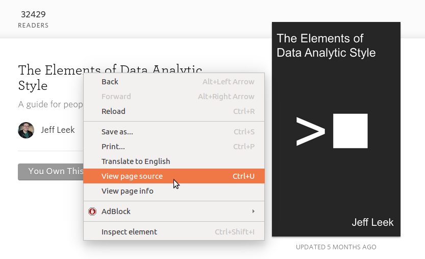
Within this portion we can see our value for the number of readers! We can examine the underlying code for a page while in a web browser. Just right click on a portion of the page and a dialogue box should appear with an option to ‘View page source…’

Armed with this information we are going to work out how to parse just the number of readers using regular expressions.

A regular expression is a special text string that describes a search pattern. We can compare regular expressions to wildcards where notations such as ‘*’ represent any number of characters. However, they are not wildcards and although there are some direct similarities, they cannot be used in the same way.

To try and make understanding the regular expression that we will use a little easier, I have broken it into three separate parts which we combine just before use.

There is the actual section of the HTML that holds the number of readers;

    $regex_actual = '<span>(.*)<\/span>';

Here we are looking for text that falls between two <span> tags that consists of a single character (.) and any number (including zero) of additional characters (*). This should find and return our number of readers.

However, because there are numerous <span> tags in the code, we want to make sure that we only extract the correct block of numbers. To do that we can define additional unique combinations of characters that occur before and / or after our numbers.

The section that appears before the span should match the following;

    $regex_pre =
        '/<ul class=\'book-details-list\'>\n<li class=\'detail\'>\n';

(The \n characters are representing new-line characters.)

The section that follows the spans will look like the following;

    $regex_apre = '\n<p>Readers<\/p>/s';

There’s a new-line followed by a paragraph tag with the word ‘Readers’ in it.

Then we combine the three strings to make our regex;

    $regex = $regex_pre.$regex_actual.$regex_apre;

I’ll be honest with you dear readers. Regular expressions are something of an art form. Those who can understand them are capable of magic that I can only wonder at and those (like myself) who are noobish can only hope to try to follow the rules in the hope that it all becomes clear in the end. Don’t despair however. Experiment a bit with the code, ask for assistance when you’re struggling (stackoverflow).

Finally we carry out our match (preg_match) and return our values in the array $title;

    preg_match($regex,$file_string,$title);
    $downloads = $title[1];

    echo $downloads." ".$books[$x][1]."<br>";

In the code above we print out the number of readers followed by the title of the book so that it appears something like the following;

31095 R Programming for Data Science
32426 The Elements of Data Analytic Style

This can be tested by either running the file from the command line;

… or by browsing to the file in a web browser.

Record

To record this data we will use a PHP script that checks the reader numbers and writes them and the book name into our MySQL database. At the same time a time stamp will be added automatically.

Our PHP script will write a group of reader numbers to the database and we will execute the program at a regular interval using cron (you can read a description of how to use the crontab (the cron-table) in the Glossary).

Database preparation

First we will set up our database table that will store our data.

Using the phpMyAdmin web interface that we set up, log on using the administrator (root) account and select the ‘measurements’ database that we created as part of the initial set-up.

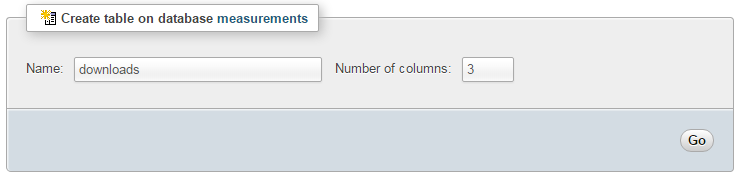
Enter in the name of the table and the number of columns that we are going to use for our measured values. In the screenshot above we can see that the name of the table is ‘downloads’ and the number of columns is ‘3’.

We will use three columns so that we can store the number of readers, the time it the number was recorded and the name of the book.

Once we click on ‘Go’ we are presented with a list of options to configure our table’s columns. Don’t be intimidated by the number of options that are presented, we are going to keep the process as simple as practical.

For the first column we can enter the name of the ‘Column’ as ‘dtg’ (short for date time group) the ‘Type’ as ‘TIMESTAMP’ and the ‘Default’ value as ‘CURRENT_TIMESTAMP’. For the second column we will enter the name ‘downloaded’ and the ‘Type’ is ‘INT’ (we won’t use a default value). For the third column we will enter the name ‘book_name’ and the type is ‘VARCHAR’ with a ‘Length/Values’ of 60.

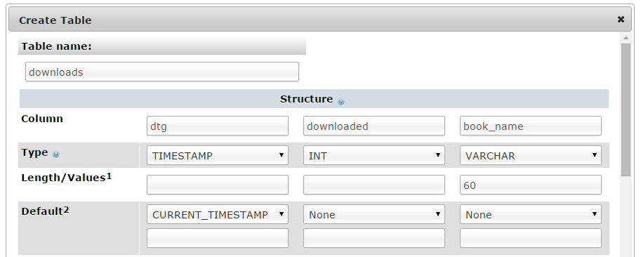
Scroll down a little and click on the ‘Save’ button and we’re done.

Record the reader numbers

The following PHP script (which is based on the code from the ‘scrape.php’ script described above) allows us to check the reader numbers from multiple books and write them to our database with a separate entry for each book.

The full code can be found in the code samples bundled with this book (scrape-book.php).

<?php

$hostname = 'localhost';
$username = 'pi_insert';
$password = 'xxxxxxxxxx';
$dbname   = 'measurements';

$books = array(
           array('https://leanpub.com/rprogramming',
                 'R Programming for Data Science'),
           array('https://leanpub.com/datastyle',
                 'The Elements of Data Analytic Style')
           );

for ($x = 0; $x <= sizeof($books)-1; $x++) {

    $file_string = file_get_contents_curl($books[$x][0]);

    $regex_pre = 
        '/<ul class=\'book-details-list\'>\n<li class=\'detail\'>\n';
    $regex_apre = '\n<p>Readers<\/p>/s';
    $regex_actual = '<span>(.*)<\/span>';
    $regex = $regex_pre.$regex_actual.$regex_apre;

    preg_match($regex,$file_string,$title);
    $downloads = $title[1];

    $link = new PDO("mysql:host=$hostname;dbname=$dbname",
                    $username,$password);

    $statement = $link->prepare(
        "INSERT INTO downloads(book_name, downloaded) VALUES(?, ?)");

    $statement->execute(array($books[$x][1], $downloads));

}

function file_get_contents_curl($url) {
    $ch = curl_init();

    curl_setopt($ch, CURLOPT_SSL_VERIFYPEER, false);
    curl_setopt($ch, CURLOPT_AUTOREFERER, TRUE);
    curl_setopt($ch, CURLOPT_HEADER, 0);
    curl_setopt($ch, CURLOPT_RETURNTRANSFER, 1);
    curl_setopt($ch, CURLOPT_URL, $url);
    curl_setopt($ch, CURLOPT_FOLLOWLOCATION, TRUE);       

    $data = curl_exec($ch);
    curl_close($ch);

    return $data;
}

?>

This script can be saved in our home directory (/home/pi) and can be run by typing;

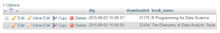
While we won’t see much happening at the command line, if we use our web browser to go to the phpMyAdmin interface and select the ‘measurements’ database and then the ‘downloads’ table we will see values of readers for the different books and their associated time of recording.

Now you can be forgiven for thinking that this is not going to collect the sort of range of data that will let us ‘Explore’ very much, but let’s do a quick explanation of the PHP script first and then we’ll work out how to record a lot more data :-).

Code Explanation

An observant reader will notice that this script is essentially a repeat of the ‘scrape.php’ script with the addition of a few lines to write the associated values to a database. Well done you! As a result, we’ll only need to explain the additional lines.

The script starts by declaring the variables needed to write the values to the database;

$hostname = 'localhost';
$username = 'pi_insert';
$password = 'xxxxxxxxxx';
$dbname   = 'measurements';

Then inside the loop that we use for reading our book names we set up the parameters for connecting to our database;

    $link = new PDO("mysql:host=$hostname;dbname=$dbname",
                    $username,$password);

We then prepare the insert statement;

    $statement = $link->prepare(
        "INSERT INTO downloads(book_name, downloaded) VALUES(?, ?)");

… and then we execute the statement;

    $statement->execute(array($books[$x][1], $downloads));

Since these lines are inside the loop going through the array, we capture a unique record of the readers of the book every time the script is run.

Recording data on a regular basis with cron

As mentioned earlier, while our code is a thing of simplicity and elegance, it only records a single entry for each book every time it is run.

What we need to implement is a schedule so that at a regular time, the program is run. This is achieved using cron via the crontab. While we will cover the requirements for this project here, you can read more about the crontab in the Glossary.

To set up our schedule we need to edit the crontab file. This is is done using the following command;

Once run it will open the crontab in the nano editor. We want to add in an entry at the end of the file that looks like the following;

@daily /usr/bin/php /home/pi/scrape-books.php

This instructs the computer that every day it will run the command /usr/bin/python /home/pi/scrape-books.php (which if we were at the command line in the pi home directory we would run as php scrape-books.php, but since we can’t guarantee where we will be when running the script, we are supplying the full path to the php command and the scrape-books.php script.

Save the file and the next time the day rotates past midnight (the default for ‘@daily’) it will run our program on its designated schedule and we will have reader numbers written to our database every day.

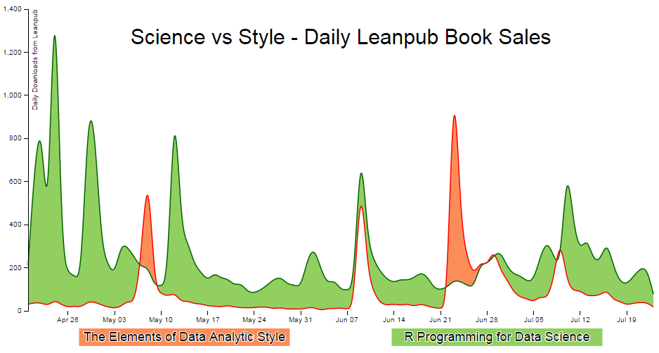
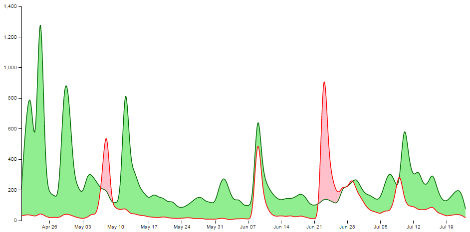
Explore

This section presents our data in a difference chart which is a variation on a bivariate area chart. This is a line chart that includes two lines that are interlinked by filling the space between the lines. A difference chart as demonstrated in the example here by Mike Bostock is able to highlight the differences between the lines by filling the area between them with different colours depending on which line is the greater value.

As Mike points out in his example, this technique harks back at least as far as William Playfair when he was describing the time series of exports and imports of Denmark and Norway in 1786.

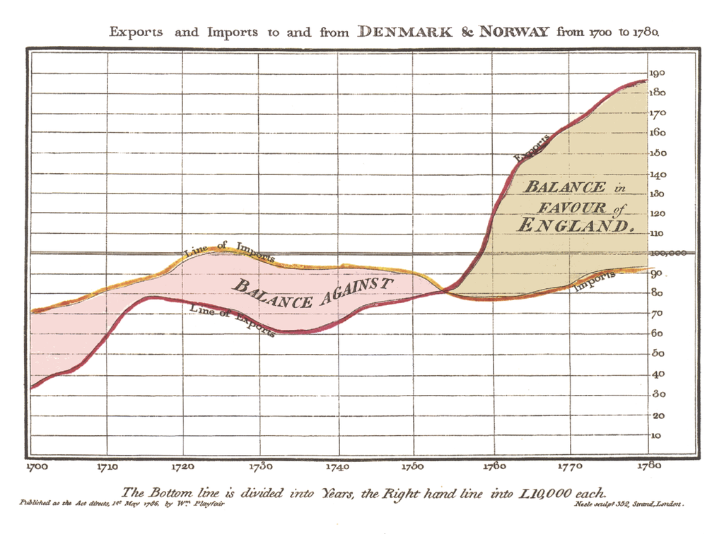
All that remains is for us to work out how d3.js can help us out by doing the job programmatically. The example that I use here is based on that of Mike Bostock’s. As an bonus extra, we will add of a few niceties in the form of a legend, a title, and some minor changes after explaining the graph.

We will start with a simple example of the code and we will add blocks to finally arrive at the example with Legends and title.

The Code

The following is the code for the simple difference chart. A live version (that imports a csv file) is available online at bl.ocks.org or GitHub. The version used here is available as the file ‘scrape-diff.php’ as a download with the book Raspberry Pi: Measure, Record, Explore (in a zip file) when you download the book from Leanpub.

<?php

$hostname = 'localhost';
$username = 'pi_select';
$password = 'xxxxxxxxxx';

try {
    $dbh = new PDO("mysql:host=$hostname;dbname=measurements",
                               $username, $password);

    /*** The SQL SELECT statement ***/

    $sth = $dbh->prepare("
SELECT *
FROM  downloads
ORDER BY  dtg, book_name
    ");
    $sth->execute();

    /* Fetch all of the remaining rows in the result set */
    $result = $sth->fetchAll(PDO::FETCH_ASSOC);

    /*** close the database connection ***/
    $dbh = null;
    
}
catch(PDOException $e)
    {
        echo $e->getMessage();
    }

$json_data = json_encode($result);     

?>

<!DOCTYPE html>
<meta charset="utf-8">
<style>

body { font: 10px sans-serif;}

text.shadow {
  stroke: white;
  stroke-width: 2px;
  opacity: 0.9;
}

.axis path,
.axis line {
  fill: none;
  stroke: #000;
  shape-rendering: crispEdges;
}

.x.axis path { display: none; }

.area.above { fill: rgb(252,141,89); }
.area.below { fill: rgb(145,207,96); }

.line {
  fill: none;
  stroke: #000;
  stroke-width: 1.5px;
}

</style>
<body>
<script src="http://d3js.org/d3.v3.min.js"></script>
<script>

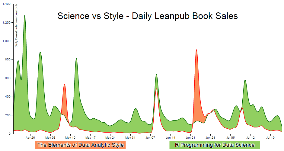
var title = "Science vs Style - Daily Leanpub Book Sales";

var margin = {top: 20, right: 20, bottom: 50, left: 50},
    width = 960 - margin.left - margin.right,
    height = 500 - margin.top - margin.bottom;

var parsedtg = d3.time.format("%Y-%m-%d %H:%M:%S").parse;

var x = d3.time.scale().range([0, width]);
var y = d3.scale.linear().range([height, 0]);

var xAxis = d3.svg.axis().scale(x).orient("bottom");
var yAxis = d3.svg.axis().scale(y).orient("left");

var lineScience = d3.svg.area()
    .interpolate("basis")
    .x(function(d) { return x(d.dtg); })
    .y(function(d) { return y(d["Science"]); });

var lineStyle = d3.svg.area()
    .interpolate("basis")
    .x(function(d) { return x(d.dtg); })
    .y(function(d) { return y(d["Style"]); });

var area = d3.svg.area()
    .interpolate("basis")
    .x(function(d) { return x(d.dtg); })
    .y1(function(d) { return y(d["Science"]); });

var svg = d3.select("body").append("svg")
    .attr("width", width + margin.left + margin.right)
    .attr("height", height + margin.top + margin.bottom)
  .append("g")
    .attr("transform",
        "translate(" + margin.left + "," + margin.top + ")");

<?php echo "dataNest=".$json_data.";" ?>

  dataNest.forEach(function(d) {
      d.dtg = parsedtg(d.dtg);
      d.downloaded = +d.downloaded;
  });

  var data = d3.nest()
      .key(function(d) {return d.dtg;})
      .entries(dataNest);

  data.forEach(function(d) {
      d.dtg = d.values[0]['dtg'];
      d["Science"] = d.values[0]['downloaded'];
      d["Style"] = d.values[1]['downloaded'];
  });

  for(i=data.length-1;i>0;i--) {
          data[i].Science   = data[i].Science  -data[(i-1)].Science ;
          data[i].Style     = data[i].Style    -data[(i-1)].Style ;
   }

  data.shift(); // Removes the first element in the array
  
    x.domain(d3.extent(data, function(d) { return d.dtg; }));
    y.domain([
//      d3.min(data, function(d) {
//          return Math.min(d["Science"], d["Style"]); }),
//      d3.max(data, function(d) {
//          return Math.max(d["Science"], d["Style"]); })
      0,1400
    ]);

    svg.datum(data);

    svg.append("clipPath")
        .attr("id", "clip-above")
      .append("path")
        .attr("d", area.y0(0));

    svg.append("clipPath")
        .attr("id", "clip-below")
      .append("path")
        .attr("d", area.y0(height));

    svg.append("path")
        .attr("class", "area above")
        .attr("clip-path", "url(#clip-above)")
        .attr("d", area.y0(function(d) { return y(d["Style"]); }));

    svg.append("path")
        .attr("class", "area below")
        .attr("clip-path", "url(#clip-below)")
        .attr("d", area.y0(function(d) { return y(d["Style"]); }));

    svg.append("path")
        .attr("class", "line")
        .style("stroke", "darkgreen")
        .attr("d", lineScience);

    svg.append("path")
        .attr("class", "line")
        .style("stroke", "red")
        .attr("d", lineStyle);

    svg.append("g")
        .attr("class", "x axis")
        .attr("transform", "translate(0," + height + ")")
        .call(xAxis);

    svg.append("g")
        .attr("class", "y axis")
        .call(yAxis);

</script>
</body>

Description

The graph has some portions that are common to the simple graphs that have been worked through in the earlier chapters.

The PHP block at the start of the code is mostly the same as our example code for our single temperature measurement project. The significant difference however is in the select statement.

SELECT *
FROM  downloads
ORDER BY  dtg, book_name

Here, all the data is to be used (hence the *) and we order by date time group and book name.

We start the HTML file, load some styling for the upcoming elements, set up the margins, time formatting scales, ranges and axes.

Because the graph is composed of two lines we need to declare two separate line functions;

var lineScience = d3.svg.area()
    .interpolate("basis")
    .x(function(d) { return x(d.dtg); })
    .y(function(d) { return y(d["Science"]); });

var lineStyle = d3.svg.area()
    .interpolate("basis")
    .x(function(d) { return x(d.dtg); })
    .y(function(d) { return y(d["Style"]); });

To fill an area we declare an area function using one of the lines as the baseline (y1) and when it comes time to fill the area later in the script we declare y0 separately to define the area to be filled as an intersection of two paths.

var area = d3.svg.area()
    .interpolate("basis")
    .x(function(d) { return x(d.dtg); })
    .y1(function(d) { return y(d["Science"]); });

In this instance we are using the green ‘Science’ line as the y1 line.

The svg area is then set up using the height, width and margin values and we load our csv files with our number of downloads for each book. We then carry out a standard forEach to ensure that the time and numerical values are formatted correctly.

Nesting the data

The data that we are starting with is stored and formatted in a way that we could reasonably expect data to be available in this instance. This mechanism makes it easier to add additional books for recording if desired.

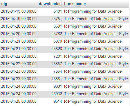
In this case, we will need to ‘pivot’ the data to produce a multi-column representation where we have a single row for each date, and the number of downloads for each book as separate columns as follows;

dtg         book 1  book 2
2015-04-19  5481    23751
2015-04-20  5691    23782
2015-04-21  6379    23820

This can be achieved using the d3 nest function.

  var data = d3.nest()
      .key(function(d) {return d.dtg;})
      .entries(dataNest);

We declare our new array’s name as data and we initiate the nest function;

	var data = d3.nest()

We assign the key for our new array as dtg. A ‘key’ is like a way of saying “This is the thing we will be grouping on”. In other words our resultant array will have a single entry for each unique date (dtg) which will have the values of the number of downloaded books associated with it.

		.key(function(d) {return d.dtg;})

Then we tell the nest function which data array we will be using for our source of data.

		}).entries(dataNest);

Wrangle the data

Once we have our pivoted data we can format it in a way that will suit the code for the visualisation. This involves storing the values for the ‘Science’ and ‘Style’ variables as part of a named index.

  data.forEach(function(d) {
      d.dtg = d.values[0]['dtg'];
      d["Science"] = d.values[0]['downloaded'];
      d["Style"] = d.values[1]['downloaded'];
  });

We then loop through the ‘Science’ and ‘Style’ array to convert the incrementing value of the total number of downloads into a value of the number that have been downloaded each day;

  for(i=data.length-1;i>0;i--) {
          data[i].Science   = data[i].Science  -data[(i-1)].Science ;
          data[i].Style     = data[i].Style    -data[(i-1)].Style ;
   }

Finally because we are adjusting from total downloaded to daily values we are left with an orphan value that we need to remove from the front of the array;

  data.shift();

Cheating with the domain

The observant d3.js reader will have noticed that the setting of the y domain has a large section commented out;

    x.domain(d3.extent(data, function(d) { return d.dtg; }));
    y.domain([
//      d3.min(data, function(d) {
//          return Math.min(d["Science"], d["Style"]); }),
//      d3.max(data, function(d) {
//          return Math.max(d["Science"], d["Style"]); })
      0,1400
    ]);

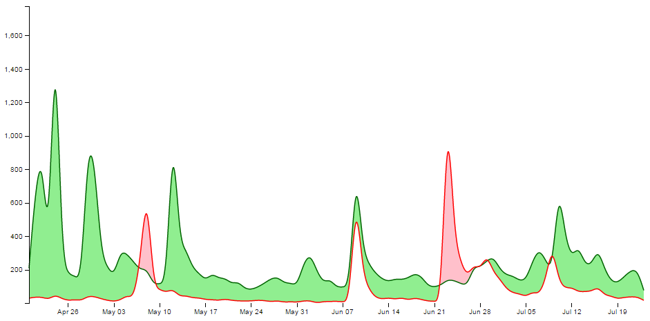
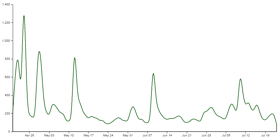
That’s because I want to be able to provide an ideal way for the graph to represent the data in an appropriate range, but because we are using the basis smoothing modifier, and the data is ‘peaky’, there is a tendency for the y scale to be fairy broad and the resultant graph looks a little lost;

Alternatively, we could remove the smoothing and let the true data be shown;

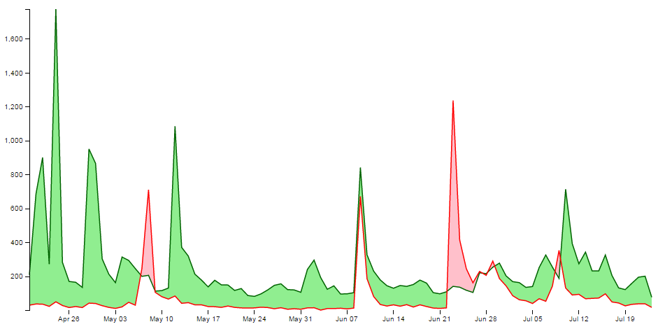
It should be argued that this is a truer representation of the data, but in this case I feel comfortable sacrificing accuracy for aesthetics (what have I become?).

Therefore, the domain for the y axis is set manually to between 0 and 1400, but feel free to remove that at the point when you introduce your own data :-).

data vs datum

One small line gets its own section. That line is;

    svg.datum(data);

A casual d3.js user could be forgiven for thinking that this doesn’t seem too fearsome a line, but it has hidden depths.

As Mike Bostock explains here, if we want to bind data to elements as a group we would be *.data, but if we want to bind that data to individual elements, we should use *.datum.

It’s a function of how the data is stored. If there is an expectation that the data will be dynamic then data is the way to go since it has the feature of preparing enter and exit selections. If the data is static (it won’t be changing) then datum is the way to go.

In our case we are assigning data to individual elements and as a result we will be using datum.

Setting up the clipPaths

The clipPath operator is used to define an area that is used to create a shape by intersecting one area with another.

In our case we are going to set up two clip paths. One is the area above the green ‘Science’ line (which we defined earlier as being the y1 component of an area selection);

This is declared via this portion of the code;

    svg.append("clipPath")
        .attr("id", "clip-above")
      .append("path")
        .attr("d", area.y0(0));

Then we set up the clip path that will exist for the area below the green ‘Science’ line ;

This is declared via this portion of the code;

    svg.append("clipPath")
        .attr("id", "clip-below")
      .append("path")
        .attr("d", area.y0(height));

Each of these paths has an ‘id’ which can be subsequently used by the following code.

Clipping and adding the areas

Now we come to clipping our shape and filling it with the appropriate colour.

We do this by having a shape that represents the area between the two lines and applying our clip path for the values above and below our reference line (the green ‘Science’ line). Where the two intersect, we fill it with the appropriate colour. The code to fill the area above the reference line is as follows;

    svg.append("path")
        .attr("class", "area above")
        .attr("clip-path", "url(#clip-above)")
        .attr("d", area.y0(function(d) { return y(d["Style"]); }));

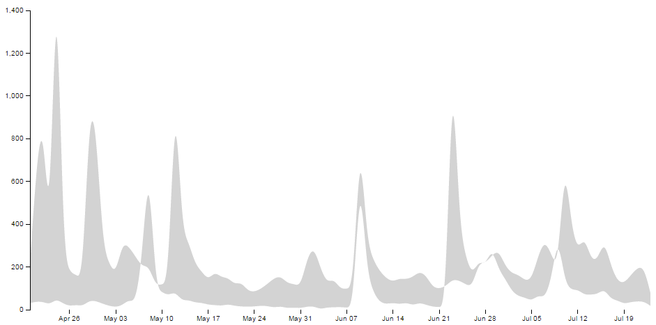
Here we have two lines that are defining the shape between the two science and style lines;

    svg.append("path")
        ....
        ....
        .attr("d", area.y0(function(d) { return y(d["Style"]); }));

If we were to look at the shape that this produces it would look as follows (greyed out for highlighting);

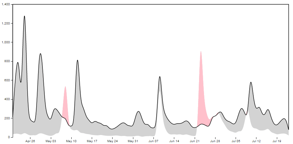
We apply a class to the shape so that is filled with the colour that we want;

        .attr("class", "area above")

.. and apply the clip path so that only the areas that intersect the two shapes are filled with the appropriate colour;

        .attr("clip-path", "url(#clip-above)")

Here the intersection of those two shapes is shown as pink;

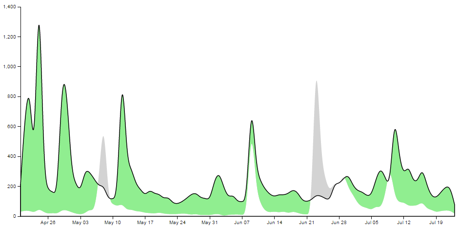
Then we do the same for the area below;

    svg.append("path")
        .attr("class", "area below")
        .attr("clip-path", "url(#clip-below)")
        .attr("d", area.y0(function(d) { return y(d["Style"]); }));

With the corresponding areas showing the intersection of the two shapes coloured differently;

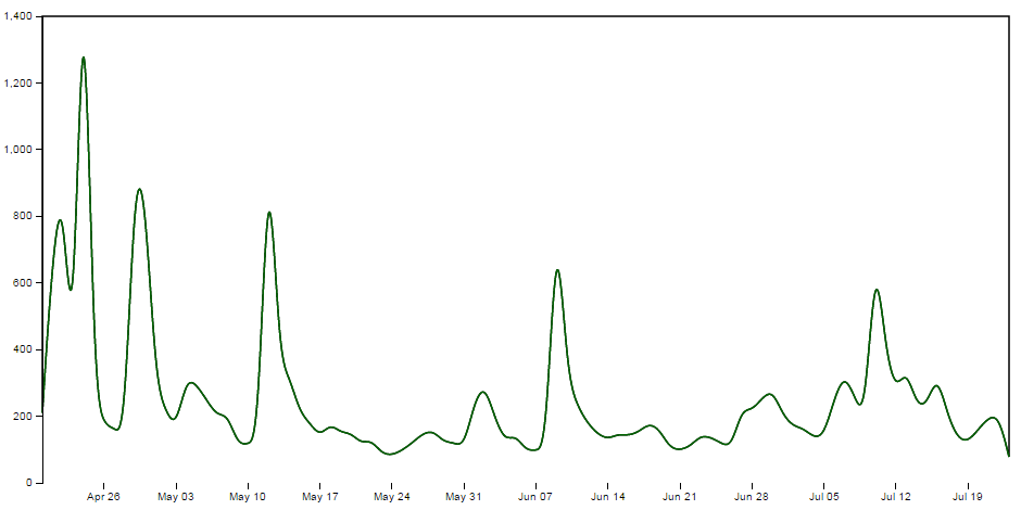
Draw the lines and the axes

The final part of our basic difference chart is to draw in the lines over the top so that they are highlighted and to add in the axes;

    svg.append("path")
        .attr("class", "line")
        .style("stroke", "darkgreen")
        .attr("d", lineScience);

    svg.append("path")
        .attr("class", "line")
        .style("stroke", "red")
        .attr("d", lineStyle);

    svg.append("g")
        .attr("class", "x axis")
        .attr("transform", "translate(0," + height + ")")
        .call(xAxis);

    svg.append("g")
        .attr("class", "y axis")
        .call(yAxis);

Et viola! we have our difference chart!

As mentioned earlier, the code for the simple difference chart using a csv data file is available online at bl.ocks.org or GitHub. It is also available as the file ‘scrape-diff.php’ as a download with the book (in a zip file) when you download the book from Leanpub.

Adding a bit more to our difference chart.

The chart itself is a thing of beauty, but given the subject matter (it’s describing two books after all) we should include a bit more information on what it is we’re looking at and provide some links so that a fascinated viewer of the graphs can read the books!

Add a Y axis label

Because it’s not immediately obvious what we’re looking at on the Y axis we should add in a nice subtle label on the Y axis;

    svg.append("g")
        .attr("class", "y axis")
        .call(yAxis)
      .append("text")
        .attr("transform", "rotate(-90)")
        .attr("y", 6)
        .attr("dy", ".71em")
        .style("text-anchor", "end")
        .text("Daily Downloads from Leanpub");

Add a title

Every graph should have a title. The following code adds this to the top(ish) centre of the chart and provides a white drop-shadow for readability;

    // ******* Title Block ********
    svg.append("text") // Title shadow
      .attr("x", (width / 2))
      .attr("y", 50 )
      .attr("text-anchor", "middle")
      .style("font-size", "30px")
      .attr("class", "shadow")
      .text(title);

    svg.append("text") // Title
      .attr("x", (width / 2))
      .attr("y", 50 )
      .attr("text-anchor", "middle")
      .style("font-size", "30px")
      .style("stroke", "none")
      .text(title);

Adding the legend

A respectable legend in this case should provide visual context of what it is describing in relation to the graph (by way of colour) and should actually name the book. We can also go a little bit further and provide a link to the books in the legend so that potential readers can access them easily.

Firstly the rectangles filled with the right colour, sized appropriately and arranged just right;

    var block = 300;   // rectangle width and position

    svg.append("rect") // Style Legend Rectangle
      .attr("x", ((width / 2)/2)-(block/2))
      .attr("y", height+(margin.bottom/2) )
      .attr("width", block)
      .attr("height", "25")
      .attr("class", "area above");

    svg.append("rect") // Science Legend Rectangle
      .attr("x", ((width / 2)/2)+(width / 2)-(block/2))
      .attr("y", height+(margin.bottom/2) )
      .attr("width", block)
      .attr("height", "25")
      .attr("class", "area below");

Then we add the text (with a drop-shadow) and a link;

    svg.append("text") // Style Legend Text shadow
      .attr("x", ((width / 2)/2))
      .attr("y", height+(margin.bottom/2) + 5)
      .attr("dy", ".71em")
      .attr("text-anchor", "middle")
      .style("font-size", "18px")
      .attr("class", "shadow")
      .text("The Elements of Data Analytic Style");

    svg.append("text") // Science Legend Text shadow
      .attr("x", ((width / 2)/2)+(width / 2))
      .attr("y", height+(margin.bottom/2) + 5)
      .attr("dy", ".71em")
      .attr("text-anchor", "middle")
      .style("font-size", "18px")
      .attr("class", "shadow")
      .text("R Programming for Data Science");

    svg.append("a")
      .attr("xlink:href", "https://leanpub.com/datastyle")
      .append("text") // Style Legend Text
      .attr("x", ((width / 2)/2))
      .attr("y", height+(margin.bottom/2) + 5)
      .attr("dy", ".71em")
      .attr("text-anchor", "middle")
      .style("font-size", "18px")
      .style("stroke", "none")
      .text("The Elements of Data Analytic Style");

    svg.append("a")
      .attr("xlink:href", "https://leanpub.com/rprogramming")
      .append("text") // Science Legend Text
      .attr("x", ((width / 2)/2)+(width / 2))
      .attr("y", height+(margin.bottom/2) + 5)
      .attr("dy", ".71em")
      .attr("text-anchor", "middle")
      .style("font-size", "18px")
      .style("stroke", "none")
      .text("R Programming for Data Science");

I’ll be the first to admit that this could be done more efficiently with some styling via css, but then it would leave nothing for the reader to try :-).

Link the areas

As a last touch we can include the links to the respective books in the shading for the graph itself;

    svg.append("a")
      .attr("xlink:href", "https://leanpub.com/datastyle")
      .append("path")
        .attr("class", "area above")
        .attr("clip-path", "url(#clip-above)")
        .attr("d", area.y0(function(d) { return y(d["Style"]); }));

    svg.append("a")
      .attr("xlink:href", "https://leanpub.com/rprogramming")
      .append("path")
        .attr("class", "area below")
        .attr("clip-path", "url(#clip-below)")
        .attr("d", area.y0(function(d) { return y(d["Style"]); }));

Perhaps not strictly required, but a nice touch none the less.

The final result

And here it is;

The code for the full difference chart using a csv file for data is available online at bl.ocks.org or GitHub. It is also available as the file ‘scrape-diff-full.php’ as a download with the book (in a zip file) when you download the book from Leanpub.