System Information Measurement
This project will measure system information that shows how our Raspberry Pi is operating. This is useful information that will allow us to monitor the performance of our computing asset and to identify potential problems before they occur (or to discover the cause of problems when they do).
Specifically we are going to measure, record and display;
- System load average
- Memory (Ram) usage
- Disk usage (on our SD card)
- Temperature of the Raspberry Pi
Measure
Hardware required
Only the Raspberry Pi! All the readings are taken from the Pi itself.
Measured Parameters
System Load
Load average is available in the file /proc/loadavg. We can print the contents of this file using cat;
This will produce a line showing five (or maybe six depending on how you look at it) pieces of information that will look a little like the following;
0.14 0.11 0.13 1/196 16991
The first three numbers give the average load for 1 minute (0.14), 5 minutes (0.11) and 15 minutes (0.13) respectively. The next combination of two numbers separated by a slash (1/196) provides two(ish) pieces of information. Firstly, the number before the slash gives the number of threads running at that moment. This should be less than or equal to the CPUs in the system and in the case of the Raspberry Pi this should be less than or equal to 1. The number after the slash indicates the total number of threads in the system. The last number is the process Id (the ‘pid’) of the thread that ran last.
We’re more interested in the system load numbers. Load average is an indication of whether the system resources (mainly the CPU) are adequately available for the processes (system load) that are running, runnable or in uninterruptible sleep states during the previous n minutes. A process is running when it has the full attention of the CPU. A runnable process is a process that is waiting for the CPU. A process is in uninterruptible sleep state when it is waiting for a resource and cannot be interrupted and will return from sleep only when the resource becomes available or a timeout occurs.
For example, a process may be waiting for disk or access to the network. Runnable processes indicate that we need more CPUs. Similarly processes in uninterruptible sleep state indicate Input/Output (I/O) bottlenecks. The load number at any time is the number of running, runnable and uninterruptible sleep state processes (we will call these collectively runnable processes) in the system. The load average is the average of the load number during the previous n minutes.
If, in a single CPU system such as our Raspberry Pi, the load average is 5, it is an undesirable situation because one process runs on the CPU and the other 4 have to wait for their turn. So the system is overloaded by 400%. In the above cat /proc/loadavg command output the load average for the last minute is 0.14, which indicates that the CPU is underloaded by 86%. Load average figures help in figuring out how much our system is able to cater to processing demands.
For our project we will record the value of system load at one of those intervals.
Memory Used
The memory being used by the Raspberry Pi can be determined using the free command. If we type in the command as follows we will see an interesting array of information;
Produces …
             total       used       free     shared    buffers     cached
Mem:           437        385         51          0         85        197
-/+ buffers/cache:        102        335
Swap:           99          0         99
This is displaying the total amount of free and used physical and swap memory in the system, as well as the buffers used by the kernel. We also used the -m switch at the end of the command to display the information in megabytes.
The row labelled ‘Mem’, displays physical memory utilization, including the amount of memory allocated to buffers and caches.
The next line of data, which begins with ‘-/+ buffers/cache’, shows the amount of physical memory currently devoted to system buffer cache. This is particularly meaningful with regards to applications, as all data accessed from files on the system pass through this cache. This cache can greatly speed up access to data by reducing or eliminating the need to read from or write to the SD card.
The last row, which begins with ‘Swap’, shows the total swap space as well as how much of it is currently in use and how much is still available.
For this project we will record the amount of memory used as a percentage of the total available.
Disk Used
It would be a useful metric to know what the status of our available hard drive space was. To determine this we can use the df command. If we use the df command without any arguments as follows;
Produces …
Filesystem     1K-blocks    Used Available Use% Mounted on
rootfs           7513804 2671756   4486552  38% /
/dev/root        7513804 2671756   4486552  38% /
devtmpfs          219744       0    219744   0% /dev
tmpfs              44784     264     44520   1% /run
tmpfs               5120       0      5120   0% /run/lock
tmpfs              89560       0     89560   0% /run/shm
/dev/mmcblk0p1     57288    9920     47368  18% /boot
The first column shows the name of the disk partition as it appears in the /dev directory. The following columns show total space, blocks allocated and blocks available. The capacity column indicates the amount used as a percentage of total file system capacity.
The final column shows the mount point of the file system. This is the directory where the file system is mounted within the file system tree. Note that the root partition will always show a mount point of /. Other file systems can be mounted in any directory of a previously mounted file system.
For our purposes the root file system (/dev/root) would be ideal. We can reduce the amount of information that we have to deal with by running the df command and requesting information on a specific area. For example…
It will produce …
Filesystem     1K-blocks    Used Available Use% Mounted on
/dev/root        7513804 2671756   4486552  38% /
In the project we will use the percentage used of the drive space as our metric.
Raspberry Pi Temperature
The Raspberry Pi includes a temperature sensor in its CPU. The reading can be found by running the command
Which will produce a nice, human readable output similar to the following;
temp=39.0'C
This value shouldn’t be taken as an indication of the ambient temperature of the area surrounding the Pi. Instead it is an indication of the temperature of the chip that contains the CPU. Monitoring this temperature could be useful since there is a maximum temperature at which it can operate reliably. Admittedly that maximum temperature is 85 degrees for the CPU (the BCM2835) and once it hits that figure it reduces the clock to reduce the temperature, but none the less, in some environments it will be a factor.
Record
To record this data we will use a Python program that checks all the the values and writes them into our MySQL database along with the current time stamp.
Our Python program will only write a single group of readings to the database and we will execute the program at a regular interval using a cron job in the same way as the multiple temperature sensor project.
Database preparation
First we will set up our database table that will store our data.
Using the phpMyAdmin web interface that we set up, log on using the administrator (root) account and select the ‘measurements’ database that we created as part of the initial set-up.
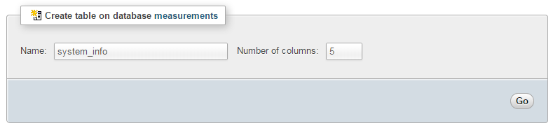
Enter in the name of the table and the number of columns that we are going to use for our measured values. In the screenshot above we can see that the name of the table is ‘system_info’ and the number of columns is ‘5’.
We will use five columns so that we can store our four readings (system load, used ram, used disk and CPU temperature).
Once we click on ‘Go’ we are presented with a list of options to configure our table’s columns. Again, we are going to keep the process as simple as practical and while we could be more economical with our data type selections, we’ll err on the side of simplicity.
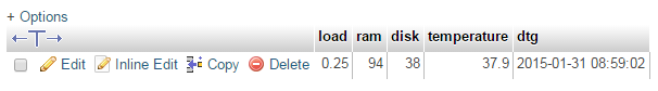
For the first column we can enter the name of the ‘Column’ as ‘load’ with a type of ‘REAL’. Our second column is ‘ram’ and our third is ‘disk’. Both of these should have a type of ‘TINYINT’. Then we have a column for ‘temperature’ and the type is ‘FLOAT’. Lastly we include the column ‘dtg’ (short for date time group) the type as ‘TIMESTAMP’ and the ‘Default’ value as ‘CURRENT_TIMESTAMP’.
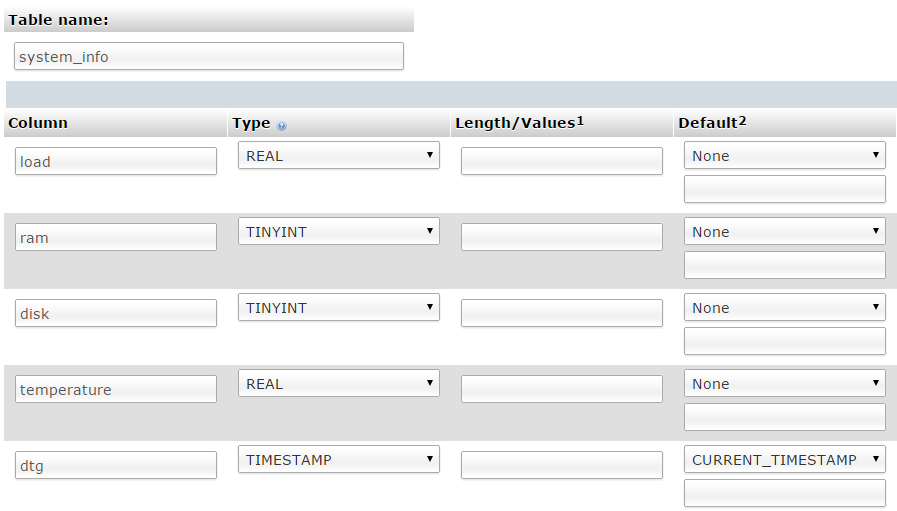
Scroll down a little and click on the ‘Save’ button and we’re done.

Record the system information values
The following Python code is a script which allows us to check the system readings from the Raspberry Pi and writes them to our database.
The full code can be found in the code samples bundled with this book (system_info.py).
#!/usr/bin/python
# -*- coding: utf-8 -*-

import subprocess
import os
import MySQLdb as mdb

# Function for storing readings into MySQL
def insertDB(system_load, ram, disk, temperature):

  try:
    con = mdb.connect('localhost',
                      'pi_insert',
                      'xxxxxxxxxx',
                      'measurements');
    cursor = con.cursor()

    sql = "INSERT INTO system_info(`load`,`ram`,`disk`,`temperature`) \
    VALUES ('%s', '%s', '%s', '%s')" % \
    (system_load, ram, disk, temperature)
    cursor.execute(sql)
    con.commit()

    con.close()

  except mdb.Error, e:
    con.rollback()
    print "Error %d: %s" % (e.args[0],e.args[1])
    sys.exit(1)

# returns the system load over the past minute
def get_load():
    try:
        s = subprocess.check_output(["cat","/proc/loadavg"])
        return float(s.split()[0])
    except:
        return 0

# Returns the used ram as a percentage of the total available
def get_ram():
    try:
        s = subprocess.check_output(["free","-m"])
        lines = s.split("\n")
        used_mem = float(lines[1].split()[2])
        total_mem = float(lines[1].split()[1])
        return (int((used_mem/total_mem)*100))
    except:
        return 0

# Returns the percentage used disk space on the /dev/root partition
def get_disk():
    try:
        s = subprocess.check_output(["df","/dev/root"])
        lines = s.split("\n")
        return int(lines[1].split("%")[0].split()[4])
    except:
        return 0

# Returns the temperature in degrees C of the CPU
def get_temperature():
    try:
        dir_path="/opt/vc/bin/vcgencmd"
        s = subprocess.check_output([dir_path,"measure_temp"])
        return float(s.split("=")[1][:-3])
    except:
        return 0

got_load = str(get_load())
got_ram = str(get_ram())
got_disk = str(get_disk())
got_temperature = str(get_temperature())

insertDB(got_load, got_ram, got_disk, got_temperature)
This script can be saved in our home directory (/home/pi) and can be run by typing;
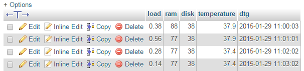
While we won’t see much happening at the command line, if we use our web browser to go to the phpMyAdmin interface and select the ‘measurements’ database and then the ‘system_info’ table we will see a range of information for the different system parameters and their associated time of reading.
As with our previous project recording multiple temperature points, this script only records a single line of data whenever it is run. To make the collection more regular we will put in a cron job later to regularly check and record.
Code Explanation
The script starts by importing the modules that it’s going to use for the process of reading and recording the temperature measurements;
import subprocess
import os
import MySQLdb as mdb
We then declare the function that will insert the readings into the MySQL database;
def insertDB(system_load, ram, disk, temperature):

  try:
    con = mdb.connect('localhost',
                      'pi_insert',
                      'xxxxxxxxxx',
                      'measurements');
    cursor = con.cursor()

    sql = "INSERT INTO system_info(`load`,`ram`,`disk`,`temperature`) \
    VALUES ('%s', '%s', '%s', '%s')" % \
    (system_load, ram, disk, temperature)
    cursor.execute(sql)
    con.commit()

    con.close()

  except mdb.Error, e:
    con.rollback()
    print "Error %d: %s" % (e.args[0],e.args[1])
    sys.exit(1)
This is a fairly simple insert of the values we will be collecting into the database.
Then we have our four functions that collect our system information;
load
As described in the earlier section we will be extracting information out of the /proc/loadavg file. Specifically we will extract the average load for the last minute. We are going to accomplish this using the following code;
def get_load():
    try:
        s = subprocess.check_output(["cat","/proc/loadavg"])
        return float(s.split()[0])
    except:
        return 0
The code employs the subprocess module (which we loaded at the start of the script) which in this case is using the check_output convenience function which will run the command (cat) and the argument (/proc/loadavg). It will return the output as a string (0.14 0.11 0.13 1/196 16991) that we can then manipulate. This string is stored in the variable s.
The following line returns the value from the function. The value is a floating number (decimal) and we are taking the first part (split()[0]) of the string (s) which by default is being split on any whitespace. In the case of our example string (0.14 0.11 0.13 1/196 16991) that would return the value 0.14.
If there is a problem retrieving the number it will be set to 0 (except: return 0).
ram
As described in the earlier section we will be extracting information out of the results from running the free command with the -m argument. Specifically we will extract the used memory and total memory values and convert them to a percentage. We are going to accomplish this using the following code;
def get_ram():
    try:
        s = subprocess.check_output(["free","-m"])
        lines = s.split("\n")
        used_mem = float(lines[1].split()[2])
        total_mem = float(lines[1].split()[1])
        return (int((used_mem/total_mem)*100))
    except:
        return 0
The code employs the subprocess module (which we loaded at the start of the script) which in this case is using the check_output convenience function which will run the command (free) and the argument (-m). It will store the returned multi-line output showing memory usage in the variable s. The output from this command (if it is run from the command line) would look a little like this;
             total       used       free     shared    buffers     cached
Mem:           437        385         51          0         85        197
-/+ buffers/cache:        102        335
Swap:           99          0         99
We then split that output string line by line and store the result in the array lines using lines = s.split("\n").
Then we find the used and total memory by looking at the second line down (lines[1]) and extracting the appropriate column (split()[2] for used and split()[1] for total).
Then it’s just some simple math to turn the memory variables (used_mem and total_mem) into a percentage.
If there is a problem retrieving the number it will be set to 0 (except: return 0).
disk
As described in the earlier section we will be extracting information out of the results from running the df command with the /dev/root argument. Specifically we will extract the percentage used value. We will accomplish this using the following code;
def get_disk():
    try:
        s = subprocess.check_output(["df","/dev/root"])
        lines = s.split("\n")
        return int(lines[1].split("%")[0].split()[4])
    except:
        return 0
The code employs the subprocess module (which we loaded at the start of the script) which in this case is using the check_output convenience function which will run the command (df) and the argument (/dev/root). It will store the returned multi-line output showing disk partition usage data in the variable s.
We then split that output string line by line and store the result in the array lines using lines = s.split("\n").
Then, using the second line down (lines[1])…
/dev/root 7513804 2671756 4486552 38% /
… we extracting the percentage column (split()[4]) and remove the percentage sign from the number (split("%")[0]). The final value is returned as an integer.
If there is a problem retrieving the number it will be set to 0 (except: return 0).
temperature
As described in the earlier section we will be extracting the temperature of the Raspberry Pis CPU the vcgencmd command with the measure_temp argument. We will accomplish this using the following code;
def get_temperature():
    try:
        dir_path="/opt/vc/bin/vcgencmd"
        s = subprocess.check_output([dir_path,"measure_temp"])
        return float(s.split("=")[1][:-3])
    except:
        return 0
The code employs the subprocess module (which we loaded at the start of the script) which in this case is using the check_output convenience function which will run the command (vcgencmd) and the argument (/dev/root) The vcgencmd command is referenced by its full path name which is initially stored as the variable dir_path and is then used in the subprocess command (this is only done for the convenience of not causing a line break in the code for the book by the way). The measure_temp argument returns the temperature in a human readable string (temp=39.0'C) which is stored in the variable s.
We are extracting the percentage value by splitting the line on the equals sign (split("=")), taking the text after the equals sign and trimming off the extra that is not required ([1][:-3]). The final value is returned as an real number.
If there is a problem retrieving the number it will be set to 0 (except: return 0).
Main program
The main part of the program (if you can call it that) consists of only the following lines;
got_load = str(get_load())
got_ram = str(get_ram())
got_disk = str(get_disk())
got_temperature = str(get_temperature())

insertDB(got_load, got_ram, got_disk, got_temperature)
They serve to retrieve the value from each of our measurement functions and to then send the results to the function that writes the values to the database.
Recording data on a regular basis with cron
As mentioned earlier, while our code is a thing of beauty, it only records a single entry for each sensor every time it is run.
What we need to implement is a schedule so that at a regular time, the program is run. This is achieved using cron via the crontab. While we will cover the requirements for this project here, you can read more about the crontab in the Glossary.
To set up our schedule we need to edit the crontab file. This is is done using the following command;
Once run it will open the crontab in the nano editor. We want to add in an entry at the end of the file that looks like the following;
*/1 * * * * /usr/bin/python /home/pi/system_info.py
This instructs the computer that every minute of every hour of every day of every month we run the command /usr/bin/python /home/pi/system_info.py (which if we were at the command line in the pi home directory we would run as python system_info.py, but since we can’t guarantee where we will be when running the script, we are supplying the full path to the python command and the system_info.py script.
Save the file and the computer will start running the program on its designated schedule and we will have sensor entries written to our database every minute.
Explore
This section has a working solution for presenting real-time, dynamic information from your Raspberry Pi. This is an interesting visualization, because it relies on two scripts in order to work properly. One displays the graphical image in our browser, and the other determines the current state of the data from our Pi, or more specifically from our database. The browser is set up to regularly interrogate our data gathering script to get the values as they change. This is an effective demonstration of using dynamic visual effects with changing data.
The final form of the graph should look something like the following;
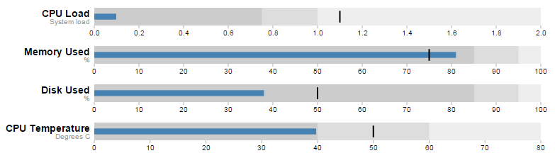
The Bullet Graph
One of the first d3.js examples I ever came across (back when it was called Protovis) was one with bullet charts (or bullet graphs). They struck me straight away as an elegant way to represent data by providing direct information and context. With it we are able to show a measured value, labelling (and sub-labels), ranges and specific markers. As a double bonus it is a relatively simple task to get them to update when our data changes. If you are interested in seeing a bit more of an overview with some examples, check out the book ‘D3 Tips and Tricks’.
The Bullet Graph Design Specification was laid down by Stephen Frew as part of his work with Perceptual Edge.
Using his specification we can break down the components of the chart as follows.
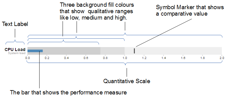
Text label:
Identifies the performance measure (the specific measured value) being represented.
Quantitative scale:
A scale that is an analogue of the scale on the x axis of a two dimensional xy graph.
Performance measure:
The specific measured value being displayed. In this case the system load on our CPU.
Comparative marker:
A reference symbol designating a measurement such as the previous day’s high value (or similar).
Qualitative ranges:
These represent ranges such as low, medium and high or bad, satisfactory and good. Ideally there would be no fewer than two and no more than 5 of these (for the purposes of readability).
Understanding the specification for the chart is useful, because it’s also reflected in the way that the data for the chart is structured.
For instance, If we take the CPU load example above, the data can be presented (in JSON) as follows;
[
  {
    "title":"CPU Load",
    "subtitle":"System Load",
    "ranges":[0.75,1,2],
    "measures":[0.17],
    "markers":[1.1]
  }
]
Here we an see all the components for the chart laid out and it’s these values that we will load into our D3 script to display.
The Code
As was outlined earlier, the code comes in two parts. The HTML / JavaScript display code and the PHP gather the data code.
First we’ll look at the HTML web page.
HTML / JavaScript
We’ll move through the explanation of the code in a similar process to the other examples in the book. Where there are areas that we have covered before, I will gloss over some details on the understanding that you will have already seen them explained in an earlier section. This code can be downloaded as sys_info.html with the code examples available with the book.
Here is the full code
<!DOCTYPE html>
<meta charset="utf-8">
<style>
<style>

body {
  font-family: "Helvetica Neue", Helvetica, Arial, sans-serif;
  margin: auto;
  padding-top: 40px;
  position: relative;
  width: 800px;
}

.bullet { font: 10px sans-serif; }
.bullet .marker { stroke: #000; stroke-width: 2px; }
.bullet .tick line { stroke: #666; stroke-width: .5px; }
.bullet .range.s0 { fill: #eee; }
.bullet .range.s1 { fill: #ddd; }
.bullet .range.s2 { fill: #ccc; }
.bullet .measure.s0 { fill: steelblue; }
.bullet .title { font-size: 14px; font-weight: bold; }
.bullet .subtitle { fill: #999; }

</style>
<script src="http://d3js.org/d3.v3.min.js"></script>
<script src="bullet.js"></script>
<script>

var margin = {top: 5, right: 40, bottom: 20, left: 130},
    width = 800 - margin.left - margin.right,
    height = 50 - margin.top - margin.bottom;

var chart = d3.bullet()
    .width(width)
    .height(height);

d3.json("sys_info.php", function(error, data) {
  var svg = d3.select("body").selectAll("svg")
      .data(data)
    .enter().append("svg")
      .attr("class", "bullet")
      .attr("width", width + margin.left + margin.right)
      .attr("height", height + margin.top + margin.bottom)
    .append("g")
      .attr("transform",
            "translate(" + margin.left + "," + margin.top + ")")
      .call(chart);

  var title = svg.append("g")
      .style("text-anchor", "end")
      .attr("transform", "translate(-6," + height / 2 + ")");

  title.append("text")
      .attr("class", "title")
      .text(function(d) { return d.title; });

  title.append("text")
      .attr("class", "subtitle")
      .attr("dy", "1em")
      .text(function(d) { return d.subtitle; });

  setInterval(function() {
    updateData();
	}, 60000);

});

function updateData() {
    d3.json("sys_info.php", function(error, data) {
        d3.select("body").selectAll("svg").datum(function (d, i) {
            d.ranges = data[i].ranges;
            d.measures = data[i].measures;
            d.markers = data[i].markers;
            return d;})
            .call(chart.duration(1000));
    });
}

</script>
</body>
The first block of our code is the start of the file and sets up our HTML.
<!DOCTYPE html>
<meta charset="utf-8">
<style>
This leads into our style declarations.
body {
  font-family: "Helvetica Neue", Helvetica, Arial, sans-serif;
  margin: auto;
  padding-top: 40px;
  position: relative;
  width: 800px;
}

.bullet { font: 10px sans-serif; }
.bullet .marker { stroke: #000; stroke-width: 2px; }
.bullet .tick line { stroke: #666; stroke-width: .5px; }
.bullet .range.s0 { fill: #eee; }
.bullet .range.s1 { fill: #ddd; }
.bullet .range.s2 { fill: #ccc; }
.bullet .measure.s0 { fill: steelblue; }
.bullet .title { font-size: 14px; font-weight: bold; }
.bullet .subtitle { fill: #999; }
We declare the (general) styling for the chart page in the first instance and then we move on to the more interesting styling for the bullet charts.
The first line .bullet { font: 10px sans-serif; } sets the font size.
The second line sets the colour and width of the symbol marker. Feel free to play around with the values in any of these properties to get a feel for what you can do. Try this for a start;
.bullet .marker { stroke: red; stroke-width: 10px; }
We then do a similar thing for the tick marks for the scale at the bottom of the graph.
The next three lines set the colours for the fill of the qualitative ranges.
.bullet .range.s0 { fill: #eee; }
.bullet .range.s1 { fill: #ddd; }
.bullet .range.s2 { fill: #ccc; }
You can have more or fewer ranges set here, but to use them you also need the appropriate values in your data file. We will explore how to change this later.
The next line designates the colour for the value being measured.
.bullet .measure.s0 { fill: steelblue; }
Like the qualitative ranges, we can have more of them, but in my personal opinion, it starts to get a bit confusing.
The final two lines lay out the styling for the label.
The next block of code loads the JavaScript files.
<script src="http://d3js.org/d3.v3.min.js"></script>
<script src="bullet.js"></script>
In this case it’s d3 and bullet.js. We need to load bullet.js as a separate file since it exists outside the code base of the d3.js ‘kernel’. The file itself can be found here and it is part of a wider group of plugins that are used by d3.js. Place the file in the same directory as the sys_info.html page for simplicities sake.
Then we get into the JavaScript. The first thing we do is define the size of the area that we’ll be working in.
var margin = {top: 5, right: 40, bottom: 20, left: 130},
    width = 800 - margin.left - margin.right,
    height = 50 - margin.top - margin.bottom;
Then we define the chart size using the variables that we have just set up.
var chart = d3.bullet()
    .width(width)
    .height(height);
The other important thing that occurs while setting up the chart is that we use the d3.bullet function call to do it. The d3.bullet function is the part that resides in the bullet.js file that we loaded earlier. The internal workings of bullet.js are a window into just how developers are able to craft extra code to allow additional functionality for d3.js.
Then we load our JSON data with our external script (which we haven’t explained yet) called sys_info_php. As a brief spoiler, sys_info.php is a script that will query our database and return the latest values in a JSON format. Hence, when it is called as below, it will provide correctly formatted data.
d3.json("sys_info.php", function(error, data) {
The next block of code is the most important IMHO, since this is where the chart is drawn.
var svg = d3.select("body").selectAll("svg")
    .data(data)
  .enter().append("svg")
    .attr("class", "bullet")
    .attr("width", width + margin.left + margin.right)
    .attr("height", height + margin.top + margin.bottom)
  .append("g")
    .attr("transform",
          "translate(" + margin.left + "," + margin.top + ")")
    .call(chart);
However, to look at it you can be forgiven for wondering if it’s doing anything at all.
We use our .select and .selectAll statements to designate where the chart will go (d3.select("body").selectAll("svg")) and then load the data as data (.data(data)).
We add in a svg element (.enter().append("svg")) and assign the styling from our css section (.attr("class", "bullet")).
Then we set the size of the svg container for an individual bullet chart using .attr("width", width + margin.left + margin.right) and .attr("height", height + margin.top + margin.bottom).
We then group all the elements that make up each individual bullet chart with .append("g") before placing the group in the right place with .attr("transform", "translate(" + margin.left + "," + margin.top + ")").
Then we wave the magic wand and call the chart function with .call(chart); which will take all the information from our data file ( like the ranges, measures and markers values) and use the bullet.js script to create a chart.
The reason I made the comment about the process looking like magic is that the vast majority of the heavy lifting is done by the bullet.js file. Because it’s abstracted away from the immediate code that we’re writing, it looks simplistic, but like all good things, there needs to be a lot of complexity to make a process look simple.
We then add the titles.
  var title = svg.append("g")
      .style("text-anchor", "end")
      .attr("transform", "translate(-6," + height / 2 + ")");

  title.append("text")
      .attr("class", "title")
      .text(function(d) { return d.title; });

  title.append("text")
      .attr("class", "subtitle")
      .attr("dy", "1em")
      .text(function(d) { return d.subtitle; });
We do this in stages. First we create a variable title which will append objects to the grouped element created above (var title = svg.append("g")). We apply a style (.style("text-anchor", "end")) and transform to the objects (.attr("transform", "translate(-6," + height / 2 + ")");).
Then we append the title and subtitle data (from our JSON file) to our chart with a modicum of styling and placement.
Lastly (inside the main part of the code) we set up a repeating function that calls another function (updateData) every 60000ms. (every minute)
  setInterval(function() {
		updateData();
	}, 60000);
Lastly we declare the function (updateData) which reads in our JSON file again, selects all the svg elements then updates all the .ranges, .measures and .markers data with whatever was in the file. Then it calls the chart function that updates the bullet charts (and it lets the change take 1000 milliseconds).
function updateData() {
	d3.json("sys_info.php", function(error, data) {
		d3.select("body").selectAll("svg")
			.datum(function (d, i) {
				d.ranges = data[i].ranges;
				d.measures = data[i].measures;
				d.markers = data[i].markers;
				return d;
			})
			.call(chart.duration(1000));
	});
}
PHP
As mentioned earlier, our html code requires JSON formatted data to be gathered and we have named the file that will do this job for us sys_info.php. This file is per the code below and it can be downloaded as sys_info.php with the downloads available with the book.
We will want to put this code in the same directory as the sys_info.py and bullet.js files, so they can find each other easily.
<?php

$hostname = 'localhost';
$username = 'pi_select';
$password = 'xxxxxxxxxx';

try {
    $dbh = new PDO("mysql:host=$hostname;dbname=measurements",
                               $username, $password);

    /*** The SQL SELECT statement ***/
    $sth = $dbh->prepare("
       SELECT *
       FROM `system_info`
       ORDER BY `dtg` DESC
       LIMIT 0,1
    ");
    $sth->execute();

    /* Fetch all of the remaining rows in the result set */
    $result = $sth->fetchAll(PDO::FETCH_ASSOC);

    /*** close the database connection ***/
    $dbh = null;

}
catch(PDOException $e)
    {
        echo $e->getMessage();
    }

$bullet_json[0]['title'] = "CPU Load";
$bullet_json[0]['subtitle'] = "System load";
$bullet_json[0]['ranges'] = array(0.75,1.0,2);
$bullet_json[0]['measures'] = array($result[0]['load']);
$bullet_json[0]['markers'] = array(1.1);

$bullet_json[1]['title'] = "Memory Used";
$bullet_json[1]['subtitle'] = "%";
$bullet_json[1]['ranges'] = array(85,95,100);
$bullet_json[1]['measures'] = array($result[0]['ram']);
$bullet_json[1]['markers'] = array(75);

$bullet_json[2]['title'] = "Disk Used";
$bullet_json[2]['subtitle'] = "%";
$bullet_json[2]['ranges'] = array(85,95,100);
$bullet_json[2]['measures'] = array($result[0]['disk']);
$bullet_json[2]['markers'] = array(50);

$bullet_json[3]['title'] = "CPU Temperature";
$bullet_json[3]['subtitle'] = "Degrees C";
$bullet_json[3]['ranges'] = array(40,60,80);
$bullet_json[3]['measures'] = array($result[0]['temperature']);
$bullet_json[3]['markers'] = array(50);

echo json_encode($bullet_json);

?>
The PHP block at the start of the code is mostly the same as our example code for our single temperature measurement project. The difference however is in the select statement.
       SELECT *
       FROM `system_info`
       ORDER BY `dtg` DESC
       LIMIT 0,1
It is selecting all the columns in our table, but by ordering the rows by date/time with the most recent at the top and then limiting the returned rows to only one, we get the single, latest row of data returned.
Most of the remainder of the script assigns the appropriate values to our array of data bullet_json.
If we consider the required format of our JSON data…
[
  {
    "title":"CPU Load",
    "subtitle":"System Load",
    "ranges":[0.75,1,2],
    "measures":[0.17],
    "markers":[1.1]
  }
]
…we can see that in our code, we are adding in our title…
$bullet_json[0]['title'] = "CPU Load";
… our subtitle…
$bullet_json[0]['subtitle'] = "System load";
… our ranges…
$bullet_json[0]['ranges'] = array(0.75,1.0,2);
… our system load value as returned from the MySQL query…
$bullet_json[0]['measures'] = array($result[0]['load']);
… and our marker(s).
$bullet_json[0]['markers'] = array(1.1);
This data is added for each chart that we will have displayed as a separate element in the bullet_json array.
Finally, we echo our JSON encoded data so that when sys_info.php is called, all d3.js ‘sees’ is correctly formatted data.
echo json_encode($bullet_json);
Now every 60 seconds, the d3.js code in the sys_info.html script calls the sys_info.php script that queries the MySQL database and gathers our latest system information. That information is collated and formatted and converted into a visual display that will update in a smooth ballet of motion.
As a way of testing that this portion of the code is working correctly, you can use your browser from an external computer and navigate to the sys_info.php file. This will print out the JSON values directly in your browser window.