Pressure and Temperature measurement with the BMP180

This project will use a BMP180 sensor manufactured by Bosch Sensortec to measure pressure and temperature. The connection will use the I2C communications protocol.

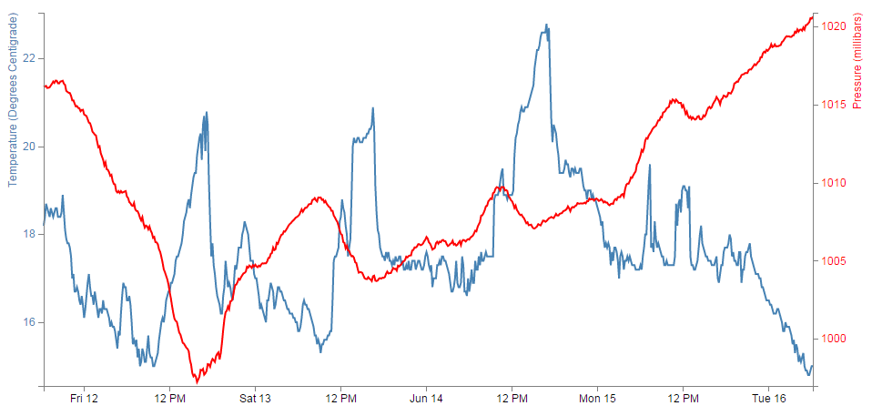
We will present the data by creating a graph with two lines representing pressure and temperature with different Y axes on the left and the right.

This project has drawn on a range of sources for information. Where not directly referenced in the text, check out the Bibliography at the end of the chapter.

Measure

Hardware required

• A Raspberry Pi (huge range of sources)
• BMP180 based sensor board. Various types are available that will perform in the same way (Adafruit, sparkfun, The Pi Hut, Deal Extreme (used in this project))
• Female to Female Dupont connector cables (Deal Extreme or build your own!)

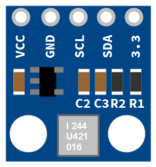
The BMP180 Sensor

The BMP180 is the a digital barometric pressure sensor made by Bosch Sensortec to support applications in mobile devices, such as smart phones, tablet PCs and sports devices. It is an improvement on an earlier device the BMP085 in terms of size and expansion of digital interfaces.

The BMP180 is a sensor based on the piezoresistive effect where a change in the electrical resistivity of a material occurs when mechanical strain is applied.

The sensor communicates using the I2C protocol and has the ability to discriminate between pressure changes corresponding to 1m in altitude and temperature changes of 0.1 degree centigrade.

Connect

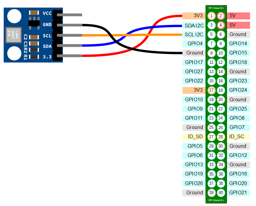
The BMP180 sensor board should be connected with ground pin to a ground connector, the 3.3 pin (or the VCC pin) to a 3.3V connector, the SCL pin to the SCL I2C connector on pin 5 and the SDA pin to the SDA I2C connector on pin 3 on the Raspberry Pi’s connector block. In the connection diagram below the ground is connected to pin 9 and the 3.3V is connected to pin 1.

This board will support a connection to the ‘VCC’ connector of 5V, but this is not advisable for the Raspberry Pi as the resulting signal levels on the SDA connector may be higher than desired for the Pi’s input. This connection can be safely used with an Arduino board.

The following diagram is a simplified view of the connection.

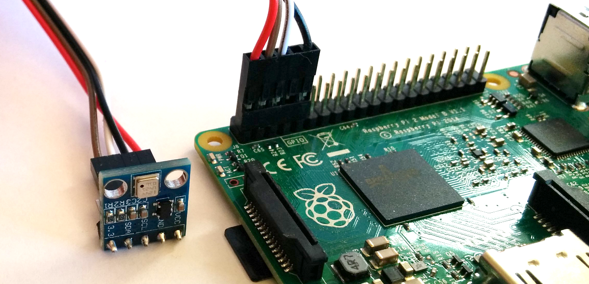
Connecting the sensor practically can be achieved in a number of ways. You could use a Pi Cobbler break out connector mounted on a bread board connected to the appropriate pins. But because the connection is relatively simple we could build a minimal configuration that will plug directly onto the pins using header connectors and jumper wire. The image below shows how simple this can be.

Test

Since the BMP180 uses the I2C protocol to communicate, we need to load the appropriate kernel support modules onto the Raspberry Pi to allow this to happen.

Firstly make sure that our software is up to date

Since we are using the Raspbian distribution there is a simple method to start the process of configuring the Pi to use the I2C protocol.

We can start by running the command;

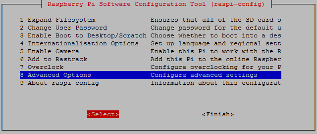
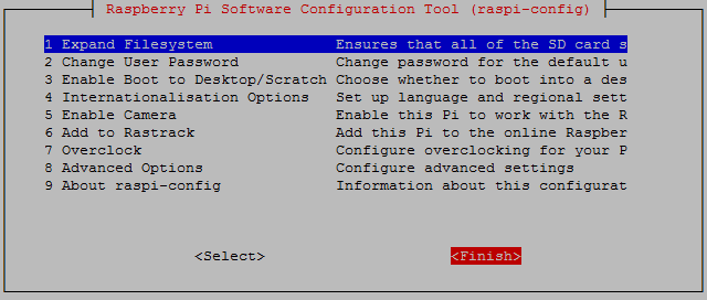
This will start the Raspberry Pi Software Configuration Tool.

On the first page select the Advanced Options with the space bar and then tab to select

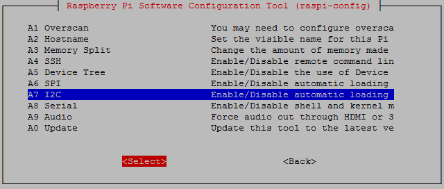
Then we select the I2C option for automatic loading of the kernel module;

Would we like the ARM I2C interface to be enabled? Yes we would;

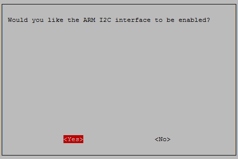
We are helpfully informed that the I2C interface will be enabled after the next reboot.

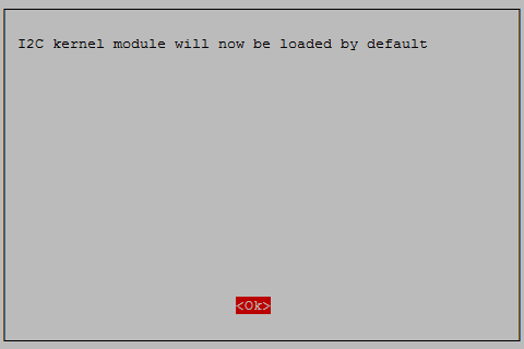
Would we like the I2C kernel module to be loaded by default? Yes we would;

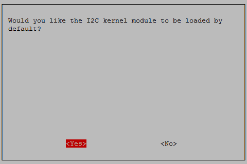
We are helpfully informed that the I2C kernel module will be loaded by default after the next reboot.

Press tab to select ‘Finish’.

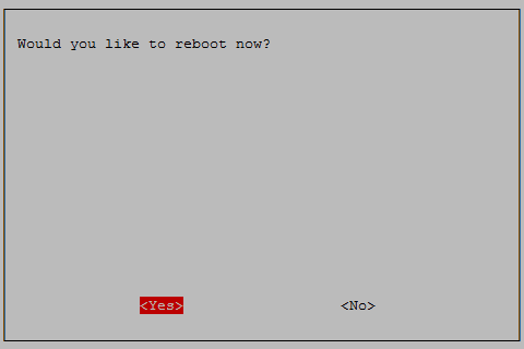
And yes, we would like to reboot.

There’s still some work to do to get things sorted. We need to edit the /etc/modules file using:

Where we need to add the following two lines to the end of the /etc/modules file:

i2c-bcm2708 
i2c-dev

Under some circumstances (depending on the kernel version we are using) we would also need to update the /boot/config.txt file. We can do this using;

Make sure that the following lines are in the file;

dtparam=i2c1=on
dtparam=i2c_arm=on

The we should load tools for working with I2C devices using the following command;

… and now we need to reboot to load the config.txt file from earlier

We can now check to see if our sensor is working using;

The output should look something like;

pi@raspberrypi ~ $ sudo i2cdetect -y 1
     0  1  2  3  4  5  6  7  8  9  a  b  c  d  e  f
00:          -- -- -- -- -- -- -- -- -- -- -- -- --
10: -- -- -- -- -- -- -- -- -- -- -- -- -- -- -- --
20: -- -- -- -- -- -- -- -- -- -- -- -- -- -- -- --
30: -- -- -- -- -- -- -- -- -- -- -- -- -- -- -- --
40: -- -- -- -- -- -- -- -- -- -- -- -- -- -- -- --
50: -- -- -- -- -- -- -- -- -- -- -- -- -- -- -- --
60: -- -- -- -- -- -- -- -- -- -- -- -- -- -- -- --
70: -- -- -- -- -- -- -- 77

This shows us that we have detected our BMP180 on channel ‘77’.

Now we want to install Python libraries designed to read the values from the BMP180. The library we are going to use was designed specifically to work with the Adafruit BMP085/BMP180 pressure sensors. In carrying out this library development, Adafruit have invested a not inconsiderable amount of time and resources. In return please consider supporting Adafruit and open-source hardware by purchasing products from Adafruit!

Now we create a directory that we will use to download the Adafruit Python library (assuming that we’re starting from our home directory);

Now we will download the library into the bmp180 directory (the following command retrieves the library from the github site);

Now that we’ve downloaded it, we need to compile it so that it can be used;

Once compilation has completed, we can test that everything has gone according to plan by running the test Python script that is installed from Github;

This will hopefully produce an output similar to the following;

Temp = 22.10 *C
Pressure = 101047.00 Pa
Altitude = 23.42 m
Sealevel Pressure = 101043.00 Pa 

The readings for the altitude and sea level pressure are both likely to be inaccurate. That’s because they are values that are calculated by the python library and not measured by the device. When the unit calculates the figures, the altitude reading requires an accurate figure for the current pressure at sea level at our location and the sea level pressure requires our altitude. Since in this simple example we never supplied either of these, the answers can hardly be expected to be accurate. Both of the currently returned figures are the results of the Adafruit_Python_BMP library using default values of 101325 Pa for sea level pressure when calculating altitude and 0 m for altitude when calculating sea level pressure.

To use values of altitude and / or sea level pressure we will want to edit the simpletest.py program that we have just run and add them in there. If we open up the file using nano we see the following towards the end of the file(or at least it will look similar to the following, I have made a small formatting change to the final line so that it doesn’t get mangled by exceeding the line width for the page);

print 'Temp = {0:0.2f} *C'.format(sensor.read_temperature())
print 'Pressure = {0:0.2f} mb'.format(sensor.read_pressure())
print 'Altitude = {0:0.2f} m'.format(sensor.read_altitude())
print 'Sealevel Pressure = {0:0.2f} Pa' \
      .format(sensor.read_sealevel_pressure())

At this point we need to know what our altitude is (in metres) and the pressure at our current location corrected to represent what it would be at seal level.

The altitude should be easy if you have a smart phone with a gps you should have a facility to use it to report it’s altitude. Let’s imagine that we have an altitude of 71m.

For the pressure we could use the map from the Weather Underground. Using the map, find the weather station closest to your location and click on it to discover what should be the corrected sea level pressure for your location.

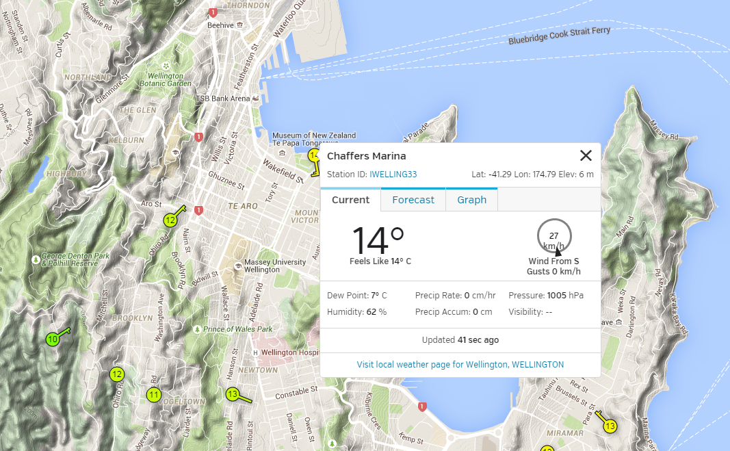
In the image above the pressure is listed as 1005hPa which is 100500Pa

Armed with the altitude and local sea level pressure we can enter them into the functions for read_altitude and read_sealevel_pressure as below;

print 'Temp = {0:0.2f} *C'.format(sensor.read_temperature())
print 'Pressure = {0:0.2f} mb'.format(sensor.read_pressure())
print 'Altitude = {0:0.2f} m'.format(sensor.read_altitude(100500))
print 'Sealevel Pressure = {0:0.2f} Pa' \
      .format(sensor.read_sealevel_pressure(71))

The next time we run the simpletest.py script we will get accurate leadings for altitude and sea level pressure. Be aware however, that these readings will only be accurate so long as the sensor does not change in altitude (don’t move it too far) or the pressure doesn’t change (and it’s always changing). So they’re useful functions (and we’ll use the seal level function in our Explore section), but we have to use them correctly.

Record

To record this data we will use a Python program that connects to our sensor, reads the values of temperature and sea level pressure and writes those values into our MySQL database. At the same time a time stamp will be added automatically.

This code will record the values when executed, but we will need to edit the crontab to allow the values to be recorded continuously (at a set interval).

Database preparation

First we will set up our database table that will store our data.

Using the phpMyAdmin web interface that we set up, log on using the administrator (root) account and select the ‘measurements’ database that we created as part of the initial set-up.

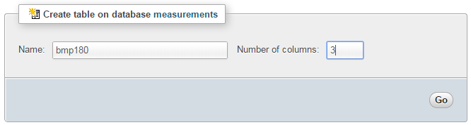
Enter in the name of the table and the number of columns that we are going to use for our measured values. In the screenshot above we can see that the name of the table is ‘bmp180’ and the number of columns is ‘3’.

We will use three columns so that we can store the temperature, pressure (the corrected sea level pressure) and the time it was recorded (‘dtg’).

Once we click on ‘Go’ we are presented with a list of options to configure our table’s columns. Don’t be intimidated by the number of options that are presented, we are going to keep the process as simple as practical.

For the first column we can enter the name of the ‘Column’ as ‘dtg’ (short for date time group) the ‘Type’ as ‘TIMESTAMP’ and the ‘Default’ value as ‘CURRENT_TIMESTAMP’. For the second column we will enter the name ‘temperature’ and the type is ‘FLOAT’. For the third column we will enter the name ‘pressure’ and the type is also ‘FLOAT’.

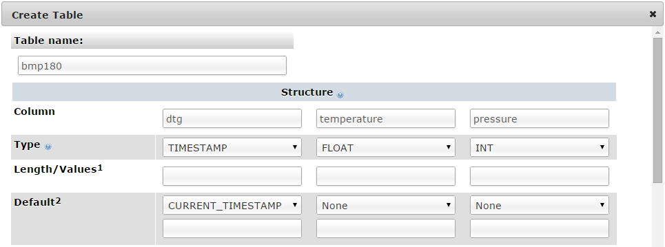
Scroll down a little and click on the ‘Save’ button and we’re done.

Record the readings

The following Python code is a script which allows us to check the state of our BMP180 sensor, return values for temperature and sea level pressure (based on a height of our sensor of 71m) and write those values to our database.

The full code can be found in the code samples bundled with this book (bmp180.py).

#!/usr/bin/python
# -*- coding: utf-8 -*-

import MySQLdb as mdb
import logging
import Adafruit_BMP.BMP085 as BMP085

# Setup logging
logging.basicConfig(filename='/home/pi/bmp180_error.log',
  format='%(asctime)s %(levelname)s %(name)s %(message)s')
logger=logging.getLogger(__name__)

# Function for storing readings into MySQL
def insertDB(temperature,pressure):

  try:

    con = mdb.connect('localhost',
                      'pi_insert',
                      'xxxxxxxxxx',
                      'measurements');
    cursor = con.cursor()

    sql = "INSERT INTO bmp180(temperature, pressure) \
    VALUES ('%s', '%s')" % \
    ( temperature, pressure)
    cursor.execute(sql)
    sql = []
    con.commit()

    con.close()

  except mdb.Error, e:
    logger.error(e)

# Get readings from sensor and store them in MySQL
sensor = BMP085.BMP085()

temperature = sensor.read_temperature()
pressure = sensor.read_sealevel_pressure(71)

insertDB(temperature,pressure)

This script can be saved in our home directory (/home/pi) as bmp180.py and can be run by typing;

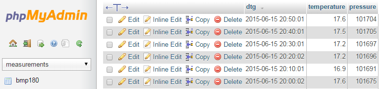
Once the command is run we should be able to check our MySQL database and see an entry for the times that the sensor was checked along with the corresponding temperature and pressure readings.

Code Explanation

The script starts by importing the modules that it’s going to use for the process of reading and recording the measurements;

import MySQLdb as mdb
import logging
import Adafruit_BMP.BMP085 as BMP085

Then the code sets up the logging module so that any failures in writing information to the database are written to the file /home/pi/bmp180_error.log.

logging.basicConfig(filename='/home/pi/bmp180_error.log',
  format='%(asctime)s %(levelname)s %(name)s %(message)s')
logger=logging.getLogger(__name__)

In the following function where we are getting our readings or writing to the database we write to the log file if there is an error. Otherwise it will accept values of temperature and pressure and write them to our database.

def insertDB(temperature,pressure):

  try:

    con = mdb.connect('localhost',
                      'pi_insert',
                      'xxxxxxxxxx',
                      'measurements');
    cursor = con.cursor()

    sql = "INSERT INTO bmp180(temperature, pressure) \
    VALUES ('%s', '%s')" % \
    ( temperature, pressure)
    cursor.execute(sql)
    sql = []
    con.commit()

    con.close()

  except mdb.Error, e:
    logger.error(e)

Which brings us to the main part of our code;

sensor = BMP085.BMP085()

temperature = sensor.read_temperature()
pressure = sensor.read_sealevel_pressure(71)

insertDB(temperature,pressure)

Here we declare our sensor (sensor = BMP085.BMP085()) then read our temperature value (sensor.read_temperature()) and pressure (sensor.read_sealevel_pressure(71)). Note here that we are including the ‘71’ as an argument for the altitude when reading the sea level pressure and therefore recording it calibrated for the height of the sensor.

Finally we call the function to insert the values into the database (insertDB(temperature,pressure)).

It’s a fairly simple block of code that is made simple by virtue of the work that has been put into the associated libraries like Adafruit_BMP.BMP085.

Recording data on a regular basis with cron

While our code is a thing of simple elegance, it only records each time it is run.

What we need to implement is a schedule so that at a regular time, the program is run. This is achieved using cron via the crontab. While we will cover the requirements for this project here, you can read more about the crontab in the Glossary.

To set up our schedule we need to edit the crontab file. This is is done using the following command;

Once run it will open the crontab in the nano editor. We want to add in an entry at the end of the file that looks like the following;

*/10 * * * * /usr/bin/python /home/pi/bmp180.py

This instructs the computer that every 10 minutes we will run the command /usr/bin/python /home/pi/bmp180.py (which if we were at the command line in the pi home directory we would run as python bmp180.py, but since we can’t guarantee where the script will be running from, we are supplying the full path to the python command and the bmp180.py script.

Save the file and the computer will start running the program on its designated schedule and we will have temperature and pressure entries written to our database every 10 minutes.

Job done! We’re measuring and recording temperature and pressure!

Explore

To explore our temperature and pressure data we will use a web based graph that shows both sets of data as lines superimposed on the same graph with separate Y axes on either side to provide value references.

The graph will be drawn using the d3.js JavaScript library and the data will be retrieved via a PHP script that queries our MySQL database.

The Code

The following code is a PHP file that we can place on our Raspberry Pi’s web server (in the /var/www directory) that will allow us to view all of the results that have been recorded in the temperature directory on a graph;

The full code can be found in the code samples bundled with this book (bmp180.php).

<?php

$hostname = 'localhost';
$username = 'pi_select';
$password = 'xxxxxxxxxx';

try {
    $dbh = new PDO("mysql:host=$hostname;dbname=measurements",
                               $username, $password);

    /*** The SQL SELECT statement ***/
    $sth = $dbh->prepare("
    SELECT `dtg` AS date,
    `temperature` AS temperature, 
    `pressure` AS pressure
    FROM `bmp180`
    ORDER BY date DESC
    LIMIT 0,900
    ");
    $sth->execute();

    /* Fetch all of the remaining rows in the result set */
    $result = $sth->fetchAll(PDO::FETCH_ASSOC);

    /*** close the database connection ***/
    $dbh = null;
}
catch(PDOException $e)
    { echo $e->getMessage(); }

$json_data = json_encode($result);      

?>

<!DOCTYPE html>
<meta charset="utf-8">
<style>

body { font: 12px Arial;}

path { 
    stroke-width: 2;
    fill: none;
}

.axis path,
.axis line {
    fill: none;
    stroke: grey;
    stroke-width: 1;
    shape-rendering: crispEdges;
}

</style>
<body>
<script src="http://d3js.org/d3.v3.min.js"></script>

<script>

var margin = {top: 30, right: 55, bottom: 30, left: 60},
    width = 960 - margin.left - margin.right,
    height = 470 - margin.top - margin.bottom;

// Parse the date / time
var parseDate = d3.time.format("%Y-%m-%d %H:%M:%S").parse;

// specify the scales for each set of data
var x = d3.time.scale().range([0, width]);
var y0 = d3.scale.linear().range([height, 0]);
var y1 = d3.scale.linear().range([height, 0]);

// axis formatting
var xAxis = d3.svg.axis().scale(x)
    .orient("bottom");
var yAxisLeft = d3.svg.axis().scale(y0)
    .orient("left").ticks(5);
var yAxisRight = d3.svg.axis().scale(y1)
    .orient("right").ticks(5).tickFormat(d3.format(".0f")); 

// line functions
var temperatureLine = d3.svg.line()
    .x(function(d) { return x(d.date); })
    .y(function(d) { return y0(d.temperature); });
var pressureLine = d3.svg.line()
    .x(function(d) { return x(d.date); })
    .y(function(d) { return y1(d.pressure); });

// seetup the svg area
var svg = d3.select("body")
    .append("svg")
        .attr("width", width + margin.left + margin.right)
        .attr("height", height + margin.top + margin.bottom)
    .append("g")
        .attr("transform", 
              "translate(" + margin.left + "," + margin.top + ")");

// Get the data
<?php echo "data=".$json_data.";" ?>

// wrangle the data into the correct formats and units
data.forEach(function(d) {
	d.date = parseDate(d.date);
	d.temperature = +d.temperature;
	d.pressure = +d.pressure/100;
});

// Scale the range of the data
x.domain(d3.extent(data, function(d) { return d.date; }));
y0.domain([
    d3.min(data, function(d) {return Math.min(d.temperature); })-.25, 
    d3.max(data, function(d) {return Math.max(d.temperature); })+.25]); 
y1.domain([
    d3.min(data, function(d) {return Math.min(d.pressure); })-.25, 
    d3.max(data, function(d) {return Math.max(d.pressure); })+.25]);

svg.append("path")      // Add the temperature line.
	.style("stroke", "steelblue")
	.attr("d", temperatureLine(data));

svg.append("path")      // Add the pressure line.
	.style("stroke", "red")
	.attr("d", pressureLine(data));

svg.append("g")         // Add the X Axis
	.attr("class", "x axis")
	.attr("transform", "translate(0," + height + ")")
	.call(xAxis);

svg.append("g")         // Add the temperature axis
	.attr("class", "y axis")
	.style("fill", "steelblue")
	.call(yAxisLeft);	

svg.append("g")         // Add the pressure axis
	.attr("class", "y axis")	
	.attr("transform", "translate(" + width + " ,0)")	
	.style("fill", "red")		
	.call(yAxisRight);

svg.append("text")      // Add the text label for the temperature axis
	.attr("transform", "rotate(-90)")
	.attr("x", 0)
	.attr("y", -30)
	.style("fill", "steelblue")
	.style("text-anchor", "end")
	.text("Temperature (Degrees Centigrade)");

svg.append("text")      // Add the text label for the pressure axis
	.attr("transform", "rotate(-90)")
	.attr("x", 0)
	.attr("y", width + 53)
	.style("fill", "red")
	.style("text-anchor", "end")
	.text("Pressure (millibars)");

</script>
</body>

This graph contains some fairly common elements that in a couple of cases are just arranged slightly differently to what we have explored in the single temperature measurement project.

The code will automatically try to collect 900 data points with a minimum time between each of 10 minutes. Depending on your requirements (any your recording times) you may want to vary the query.

PHP

The PHP block at the start of the code is mostly the same as our example code for our single temperature measurement project. The significant difference however is in the select statement.

    SELECT `dtg` AS date,
    `temperature` AS temperature, 
    `pressure` AS pressure
    FROM `bmp180`
    ORDER BY date DESC
    LIMIT 0,900

The query collects three columns of values. The Date Time Group (date), the temperature (temperature) and the pressure (pressure). There are a range of different ways that the values could be gathered and this is a very simple mechanism that grabs the latest 900 entries irrespective of the time that they were entered. In theory (so long as our bmp180.py script is working correctly) we are recording a set of readings every 10 minutes which will make for a graph that will span just over 6 days, so feel free to play about with the query to find a set of returned values that suit the data that you’re wanting to portray.

CSS (Styles)

There are a range of styles that are applied to the elements of the graphic.

body { font: 12px Arial;}

path { 
    stroke-width: 2;
    fill: none;
}

.axis path,
.axis line {
    fill: none;
    stroke: grey;
    stroke-width: 1;
    shape-rendering: crispEdges;
}

We set a default text font and size, the width and fill state for our graph lines and some formatting for our axes.

JavaScript

The code has very similar elements to our single temperature measurement script and comparing both will show us that we are doing similar things in each graph.

We set up the margins and and declare the parseDate function in much the same way as the single temperature script.

Then the first significant change occurs that will permeate through the code. Where previously we have dealt with a single Y axis, now we have to declare and differentiate between two separate Y axes. The first place that this occurs is where we scale our domains and set our ranges. This will now look like the following;

var x = d3.time.scale().range([0, width]);
var y0 = d3.scale.linear().range([height, 0]);
var y1 = d3.scale.linear().range([height, 0]);

Here y0 will serve as the scale for the temperature (on the left of the graph) and y1 will serve for pressure on the right.

Then when we declare our axes formatting functions we have to do the same thing;

var xAxis = d3.svg.axis().scale(x)
    .orient("bottom");
var yAxisLeft = d3.svg.axis().scale(y0)
    .orient("left").ticks(5);
var yAxisRight = d3.svg.axis().scale(y1)
    .orient("right").ticks(5).tickFormat(d3.format(".0f")); 

yAxisLeft uses y0 and yAxisRight uses y1. We should also note that there is a slight addition to the formatting of the right hand axis. Because the values for pressure will be over 1000 d3 will add in a comma separator for every factor of 1000. In this case I find that the comma can be a bit distracting (the largest value should in theory be only just over 1000), so the d3.format(".0f") fixes the shown values to have a fixed precision of 0 numbers after the decimal place (.0f) and by omitting the comma from the formatting statement it will not be used. For more details of formatting options in general check out the excellent page here in the D3 Wiki.

The other point of difference is that yAxisRight has the ticks orientated on the right and yAxisLeft has the ticks on the left.

Because we have two lines we need to declare two different functions for them;

var temperatureLine = d3.svg.line()
    .x(function(d) { return x(d.date); })
    .y(function(d) { return y0(d.temperature); });
var pressureLine = d3.svg.line()
    .x(function(d) { return x(d.date); })
    .y(function(d) { return y1(d.pressure); });

The SVG area is set up in the same way and then we get our data with a PHP call;

<?php echo "data=".$json_data.";" ?>

Then we cycle through our data using a forEach statement;

data.forEach(function(d) {
	d.date = parseDate(d.date);
	d.temperature = +d.temperature;
	d.pressure = +d.pressure/100;
});

In this loop we parse our date/time values so that the code knows how to use them appropriately (as time units rather than numeric values or plain text strings). Then we then do a little bit of maths to ensure that our temperature values are recognised as numbers and we divide our pressure readings (which are in pascals) by 100 so that they can be represented as millibars (since this is the more common format that people recognise and 100Pa = 1mb).

The domains for all the datasets are then established and again we need to include both Y axes;

x.domain(d3.extent(data, function(d) { return d.date; }));
y0.domain([
    d3.min(data, function(d) {return Math.min(d.temperature); })-.25, 
    d3.max(data, function(d) {return Math.max(d.temperature); })+.25]); 
y1.domain([
    d3.min(data, function(d) {return Math.min(d.pressure); })-.25, 
    d3.max(data, function(d) {return Math.max(d.pressure); })+.25]);

Here we’ve set the domain of both sets of Y axis data sets to be between the maximum and minimum of their highest and lowest values and we’ve tacked on an extra .25 to the top and bottom of the ranges to move the top and bottom of both lines just off the edges of the graph.

We then append both lines in a normal fashion and add the X and temperature axes in a familiar way. However, we do something a little different when we add the pressure axis;

svg.append("g")
	.attr("class", "y axis")	
	.attr("transform", "translate(" + width + " ,0)")	
	.style("fill", "red")		
	.call(yAxisRight);

We add in a transform attribute that moves (translates) the axis to the right hand side of the graph (using the width of the graph).

We then also utilise a transform attribute for both of the labels that we add adjacent to each Y axis. In this case however we employ the rotate operator to pivot the text so that it seems a bit more in keeping with the axis.

svg.append("text")
	.attr("transform", "rotate(-90)")
	.attr("x", 0)
	.attr("y", -30)
	.style("fill", "steelblue")
	.style("text-anchor", "end")
	.text("Temperature (Degrees Centigrade)");

svg.append("text")
	.attr("transform", "rotate(-90)")
	.attr("x", 0)
	.attr("y", width + 53)
	.style("fill", "red")
	.style("text-anchor", "end")
	.text("Pressure (millibars)");

We also move the rotated text to an appropriate position using x and y attributes. For more information on manipulating text elements with D3 check out this section from D3 Tips and Tricks.

And there we have it. Our temperature and pressure being read and presented in a stylish dual line graph.

If you want a closer explanation for this piece of code, download a copy of D3 Tips and Tricks for this and a whole swag of other information.

Bibliography

Using the BMP085/180 with Raspberry Pi or Beaglebone Black (Adafruit Learning System)

BMP180 Barometric Pressure/Temperature/Altitude Sensor- 5V ready (Adafruit Industries)

Adafruit Python library for accessing the BMP series pressure and temperature sensors (github)

BMP180 Barometric Pressure Sensor Hookup (learn.sparkfun.com)

Sensors - Pressure, Temperature and Altitude with the BMP180 (The Pi Hut)

I2C - BMP180 Temperature and Pressure Sensor (Eric Friedrich, github.com/raspberrypi-aa)

BMP180 Digital pressure sensor data sheet (Bosch)

Air pressure and wind (Eastern Illinois University)

Hypsometric equation (Wikipedia)