Setting up the Raspberry Pi
While the Raspberry Pi is a capable computer, we still need to install software on it to allow us to gather our data, store it and display it.
The software we will be using is based on the Linux Operating System. If you don’t have any familiarity with Linux, then you are about to have an exposure to it. Rest assured that we will take our time and explain things as we go. If you are a bit more confident and know your sudo from your network mask, there is a Raspberry Pi Quick Set-up section for the software loading process in the appendices.
One of the important aspects of the different projects that we are going to work on is that they have a common base. The process in the following sections will form that base, so that with each new measurement technique we take with a different sensor, we will assume that our Raspberry Pi environment has been set up with the following software. This will allow each project / chapter to be approached separately if desired.
Hardware
To make a start you will require some basic hardware to get you up and running and talking to the Raspberry Pi.
The Raspberry Pi
I know this is kind of obvious, but you will need a Raspberry Pi :-). As mentioned earlier, we will focus on using either the B+ or B2 model (they are interchangeable for the projects), but since this book is very much a living document I am hopeful that in the future we should be able to make the comparison with other models.
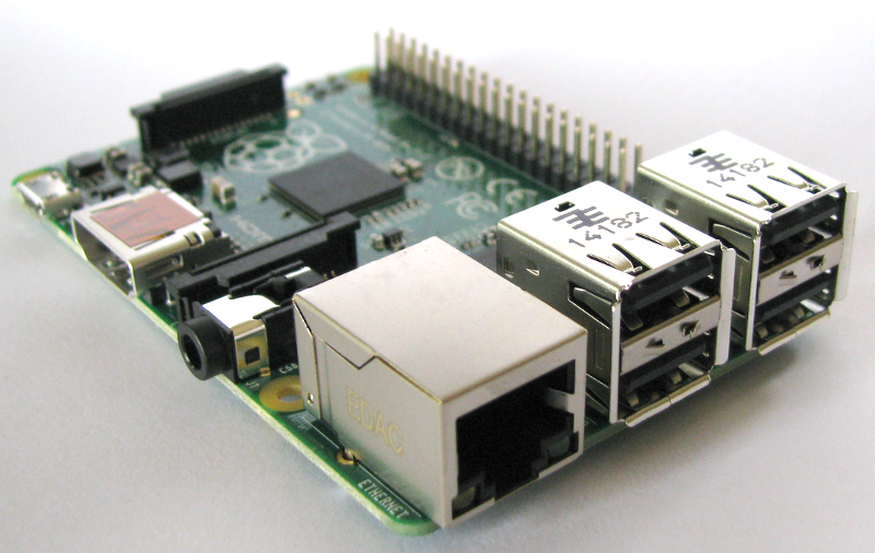
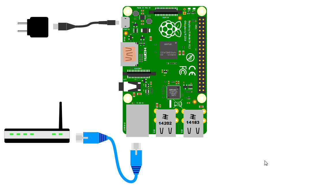
The Raspberry Pi has a great range of connection points and we will begin our set-up of the device by connecting quite a number of them to appropriate peripherals.
Case
Get yourself a simple case to sit the Pi out of the dust and detritus that’s floating about. For the purposes of ongoing development I have found that having one that leaves the top side of the Pi exposed (and the connections there accessible) is useful.
SD Card
The Raspberry Pi needs to store the Operating System and working files on a micro SD card (actually a micro SD card for the B+ model, but a full size SD card if you’re using a B model).

The microSD card receptacle is on the rear of the board and is of a ‘push-push’ type which means that you push the card in to insert it and then to remove it, give it a small push and it will spring out.
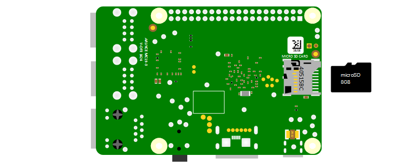
This is the equivalent of a hard drive for a regular computer, but we’re going for a minimal effect. We will want to use a minimum of an 8GB card (smaller is possible, but 8 is recommended). Also try to select a higher speed card if possible (class 10 or similar) as it is anticipated that this should speed things up a bit.
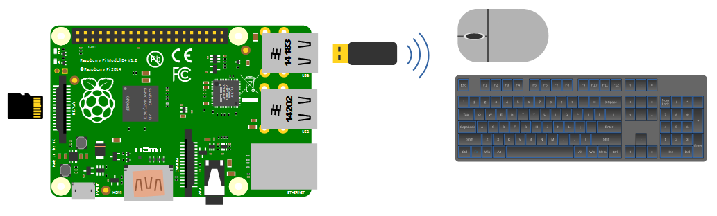
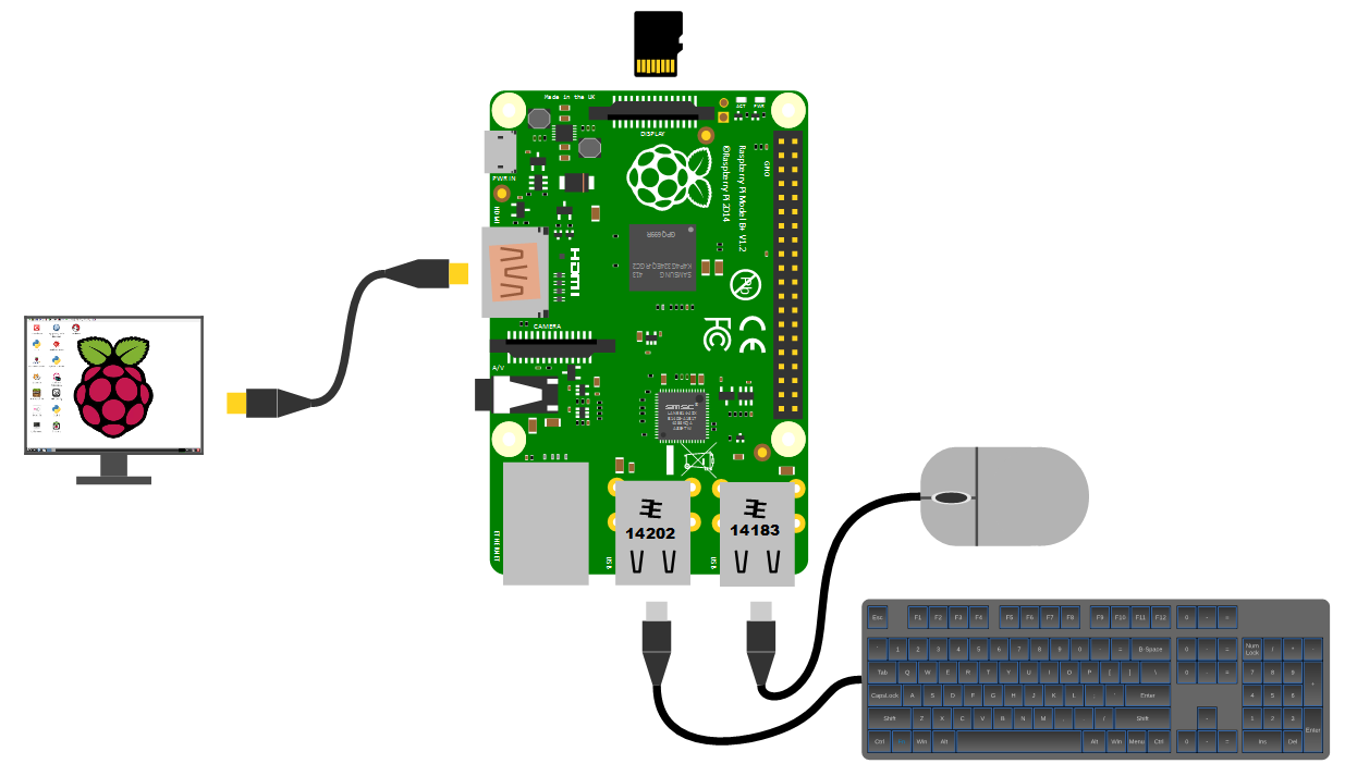
Keyboard / Mouse
While we will be making the effort to access our system via a remote computer, you will need a keyboard and a mouse for the initial set-up. Because the B+ and B2 models of the Pi have 4 x USB ports, there is plenty of space for you to connect wired USB devices.
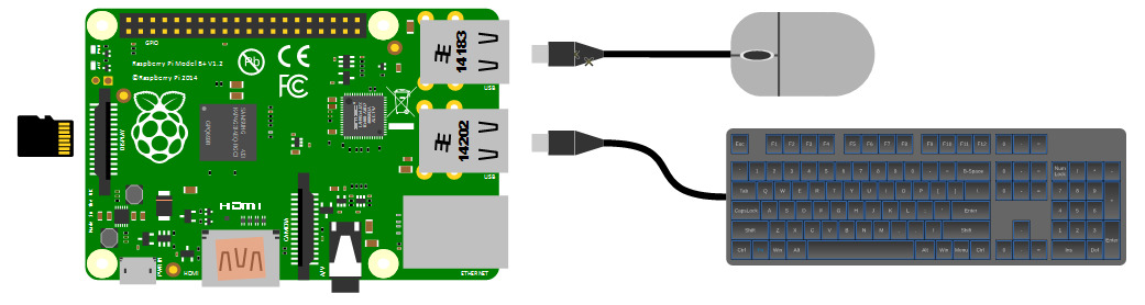
A wireless combination would most likely be recognised without any problem and would only take up a single USB port, but as we will build towards a remote capacity for using the Pi, the nicety of a wireless connection is not strictly required.
Video
The Raspberry Pi comes with an HDMI port ready to go which means that any monitor or TV with an HDMI connection should be able to connect easily.
Because this is kind of a hobby thing you might want to consider utilising an older computer monitor with a DVI or 15 pin D connector. If you want to go this way you will need an adapter to convert the connection.

Network
The B+ and B2 models of the Raspberry Pi have a standard RJ45 network connector on the board ready to go. In a domestic installation this is most likely easiest to connect into a home ADSL modem or router.
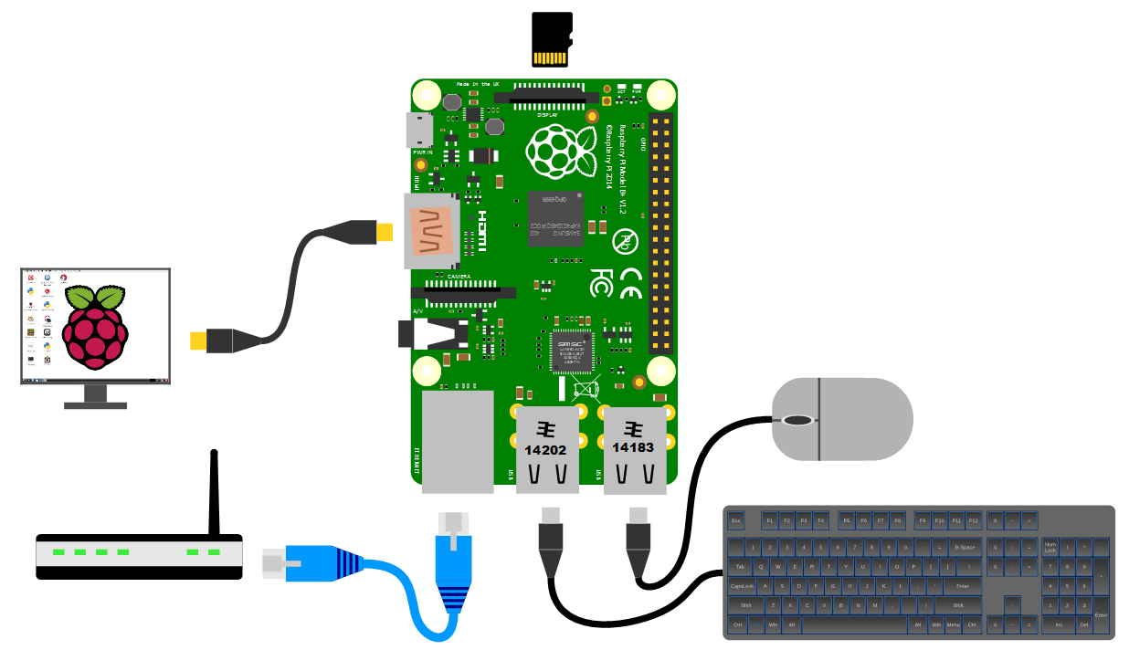
This ‘hard-wired’ connection is great for a simple start, but we will ultimately work towards a wireless solution.
Power supply
The pi can be powered up in a few ways. The simplest is to use the microUSB port to connect from a standard USB charging cable. You probably have a few around the house already for phones or tablets.
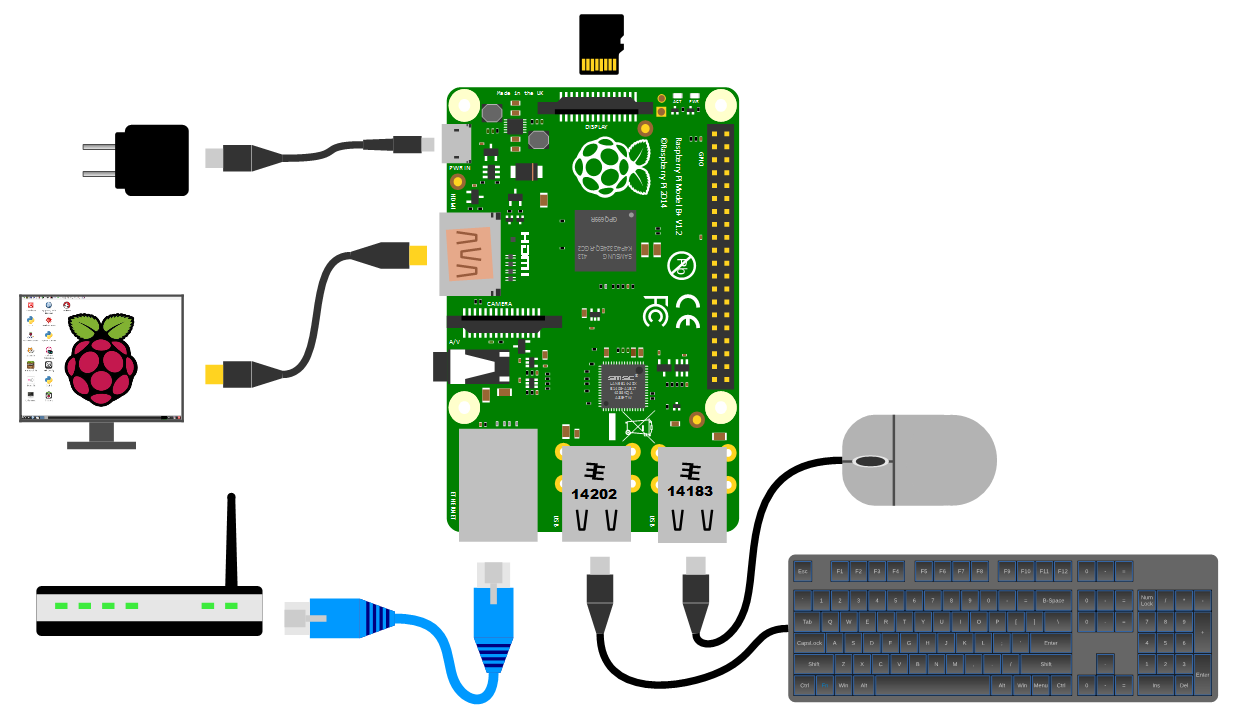
It is worth knowing that depending on what use we wish to put our Raspberry Pi to we might want to pay a certain amount of attention to the amount of current that our power supply can supply. The B+ model will function adequately with a 700mA supply, but if we want to look towards using multiple wireless devices or supplying sensors that demand power from the Pi, we should consider a supply that is capable of an output up to 2A.
Operating System
As mentioned we will be using the Linux Operating system on our Raspberry Pi. More specifically we will be installing a ‘distribution’ (version) of Linux called Raspbian.
Linux is a computer operating system that is can be distributed as free and open-source software. The defining component of Linux is the Linux kernel, an operating system kernel first released on 5 October 1991 by Linus Torvalds.
Linux was originally developed as a free operating system for Intel x86-based personal computers. It has since been made available to a huge range of computer hardware platforms and is a leading operating system on servers, mainframe computers and supercomputers. Linux also runs on embedded systems, which are devices whose operating system is typically built into the firmware and is highly tailored to the system; this includes mobile phones, tablet computers, network routers, facility automation controls, televisions and video game consoles. Android, the most widely used operating system for tablets and smart-phones, is built on top of the Linux kernel. In our case we will be using a version of Linux that is assembled to run on the ARMv6 CPU used in the Raspberry Pi.
The development of Linux is one of the most prominent examples of free and open-source software collaboration. Typically, Linux is packaged in a form known as a Linux distribution, for both desktop and server use. Popular mainstream Linux distributions include Debian, Ubuntu and the commercial Red Hat Enterprise Linux. Linux distributions include the Linux kernel, supporting utilities and libraries and usually a large amount of application software to carry out the distribution’s intended use.
A distribution intended to run as a server may omit all graphical desktop environments from the standard install, and instead include other software to set up and operate a solution stack such as LAMP (Linux, Apache, MySQL and PHP). Because Linux is freely re-distributable, anyone may create a distribution for any intended use.
Welcome to Raspbian
The Raspbian Linux distribution is based on Debian Linux. You might well be asking if that matters a great deal. Well, it kind of does since Debian is such a widely used distribution that it allows Raspbian users to leverage a huge quantity of community based experience in using and configuring the software.
Sourcing and Setting Up
On your desktop machine you are going to download the Raspbian software and write it onto the SD card. This will then be installed into the Raspberry Pi.
Downloading
The best place to source the latest version of the Raspbian Operating System is to go to the raspberrypi.org page; http://www.raspberrypi.org/downloads/.
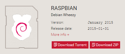
You can download via bit torrent or directly as a zip file, but whatever the method you should eventually be left with an ‘img’ file for Raspbian.
To ensure that the projects we work on can be used with either the B+ or B2 models we need to make sure that the version of Raspbian we download is from 2015-01-13 or later. Earlier downloads will not support the more modern CPU of the B2.
Writing Raspbian to the SD Card
Once we have the image file we need to get it onto our SD card.
We will work through an example using Windows 7, but for guidance on other options (Linux or Mac OS) raspberrypi.org has some great descriptions of the processes here.
We will use the Open Source utility Win32DiskImager which is available from sourceforge. This program allows us to install our Raspbian disk image onto our SD card. Download and install Win32DiskImager.
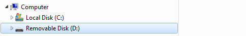
You will need an SD card reader capable of accepting your micro SD card (you may require an adapter or have a reader built into your desktop or laptop). Place the card in the reader and you should see a drive letter appear in Windows Explorer that corresponds with the SD card.
Start the Win32 Disk Imager program.
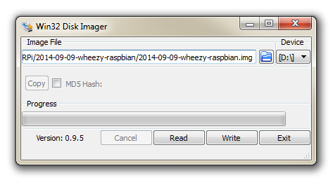
Select the correct drive letter for your SD card (make sure it’s the right one) and the Raspbian disk image that you downloaded. Then select ‘Write’ and the disk imager will write the image to the SD card. It should only take about 3-4 minutes with a class 10 SD card.
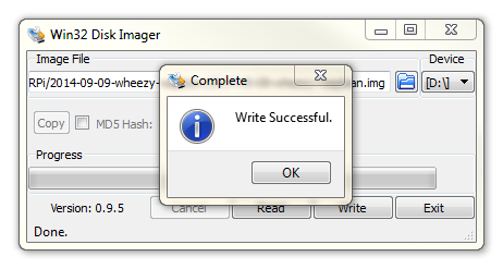
Once the process is finished exit the disk imager and eject the card from the computer and you’re done.
Installing Raspbian
Make sure that you’ve completed the previous section and have a Raspbian disk image written to a micro SD card. Insert the SD card into the slot on the Raspberry Pi and turn on the power.
You will see a range of information scrolling up the screen before eventually being presented with the Raspberry Pi Software Configuration Tool.
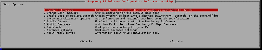
Using this tool you can first ensure that all of the SD card storage is available to the Operating System. Once this has been completed lets leave the other settings where they are for the moment and select finish. This will allow you reboot the Pi and take advantage of the full capacity of the SD card.
Once the reboot is complete you will be presented with the console prompt to log on;
Raspbian GNU/Linux 7 raspberrypi tty1

raspberrypi login:
The default username and password is:
Username: pi
Password: raspberry
Enter the username and password.
Congratulations, you have a working Raspberry Pi and are ready to start getting into the thick of things!
Firstly we’ll do a bit of house keeping.
Software Updates
The first thing we’ll do is make sure that we have the latest software for our system. This is a useful thing to do as it allows any additional improvements to the software you will be using to be enhanced or security of the operating system to be improved. This is probably a good time to mention that you will need to have an Internet connection available.
Type in the following line which will find the latest lists of available software;
You should see a list of text scroll up while the Pi is downloading the latest information.
Then we want to upgrade our software to latest versions from those lists using;
The Pi should tell you the lists of packages that it has identified as suitable for an upgrade and along with the amount of data that will be downloaded and the space that will be used on the system. It will then ask you to confirm that you want to go ahead. Tell it ‘Y’ and we will see another list of details as it heads off downloading software and installing it.
(The sudo portion of the command makes sure that you will have the permission required to run the apt-get process. For more information on the sudo command check out the Glossary here. For more on theapt-get update/upgrade commands see here)
GUI Desktop
At this point you should have found yourself staring at a screen full of text and successfully logged on to your Raspberry Pi.
You are currently working on the ‘Command Line’ or the ‘CLI’ (Command Line Interface). This is an environment that a great number of Linux users feel comfortable in and from here they are able to operate the computer in ways that can sometimes look like magic. Brace yourself… We are going to work on the command line for quite a bit while working on the Raspberry Pi. This may well be unfamiliar territory for a lot of people and to soften the blow we will also carry out a lot of our work in a Graphical User Interface (GUI).
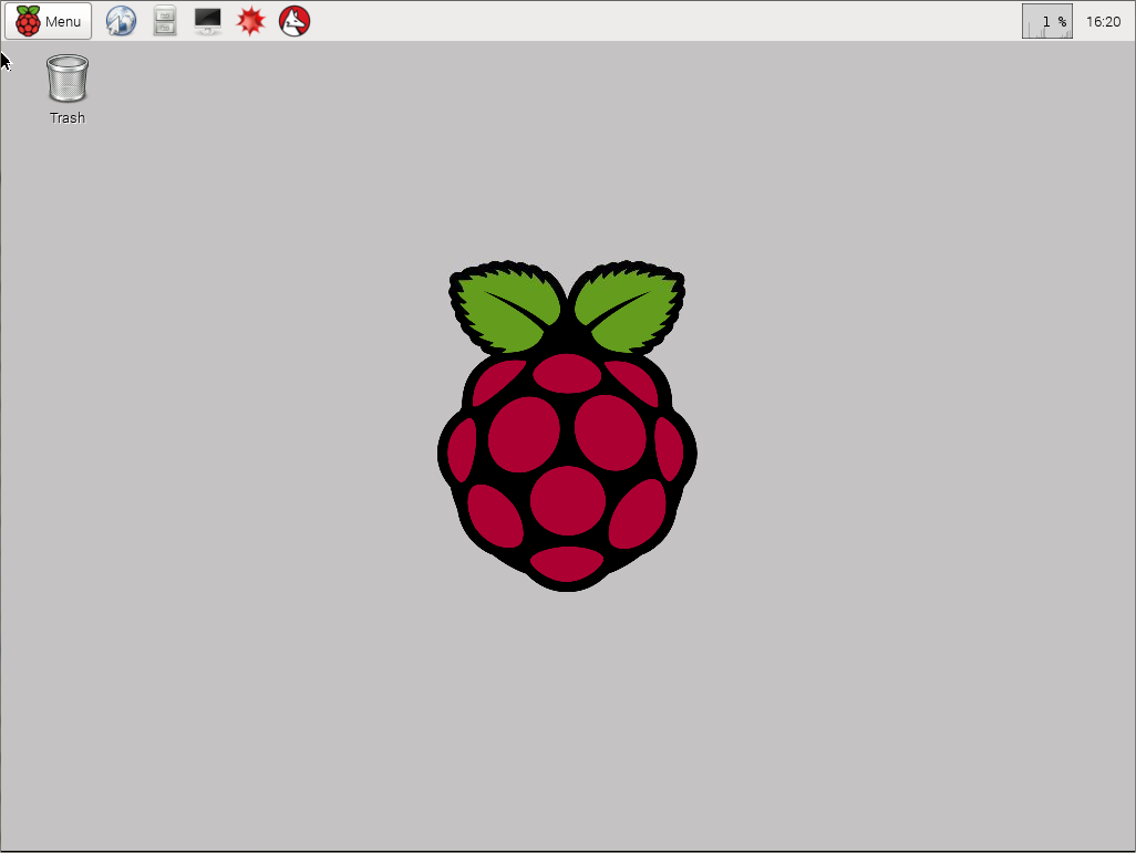
We can see what we will be using by running the command (just type it in and press return);
The command startx launches the ‘X’ session, which is to say the basic framework for a GUI environment: drawing and moving windows on the display device and interacting with a mouse and keyboard. The Raspbian distribution we are using has a desktop already set up with a range of programs ready to go that can be accessed from the menu button.
Running a GUI environment is a burden to the computer. It takes a certain degree of computing effort to maintain the graphical interface, so as a matter of course we will only us the startx command when we are wanting to interact with the computer via the desktop.
The work that we’ll be doing with the computer can be carried out in this environment without problem, but it should be envisaged that the Raspberry Pi will be tucked away somewhere out of sight and in the ideal world we wouldn’t need to be directly connected to it to interact with it. The following section describes how to configure our Pi and our desktop Windows computer so that we can remotely access the Raspberry Pi and it won’t require having a keyboard, mouse and video screen connected. Be aware however that we are going to raise the bar slightly higher in terms of computing knowledge.
Static IP Address
As noted in the previous section, enabling remote access requires that we begin to stretch ourselves slightly. In particular we will want to assign our Raspberry Pi a static IP address.
An Internet Protocol address (IP address) is a numerical label assigned to each device (e.g., computer, printer) participating in a computer network that uses the Internet Protocol for communication.
There is a strong likelihood that our Raspberry Pi already has an IP address and it should appear a few lines above the ‘login’ prompt when you first boot up;
My IP address is 10.1.1.25

Raspbian GNU/Linux 7 raspberrypi tty1

raspberrypi login:
In this example the IP address 10.1.1.25 belongs to the Raspberry Pi.
This address will probably be a ‘dynamic’ IP address and could change each time the Pi is booted. For the purposes of using the Raspberry Pi as a web platform, database and with remote access we need to set a fixed IP address.
This description of setting up a static IP address makes the assumption that we have a device running on the network that is assigning IP addresses as required. This sounds like kind of a big deal, but in fact it is a very common service to be running on even a small home network and it will be running on the ADSL modem or similar. This function is run as a service called DHCP (Dynamic Host Configuration Protocol). You will need to have access to this device for the purposes of knowing what the allowable ranges are for a static IP address. The most likely place to find a DHCP service running in a normal domestic situation would be an an ADSL modem or router.
The Netmask
A common feature for home modems and routers that run DHCP devices is to allow the user to set up the range of allowable network addresses that can exist on the network. At a higher level you should be able to set a ‘netmask’ which will do the job for you. A netmask looks similar to an IP address, but it allows you to specify the range of addresses for ‘hosts’ (in our case computers) that can be connected to the network.
A very common netmask is 255.255.255.0 which means that the network in question can have any one of the combinations where the final number in the IP address varies. In other words with a netmask of 255.255.255.0 the IP addresses available for devices on the network 10.1.1.x range from 10.1.1.0 to 10.1.1.255 or in other words any one of 256 unique addresses.
Distinguish Dynamic from Static
The other service that our DHCP server will allow is the setting of a range of addresses that can be assigned dynamically. In other words we will be able to declare that the range from 10.1.1.20 to 10.1.1.255 can be dynamically assigned which leaves 10.1.1.0 to 10.1.1.19 which can be set as static addresses.
You might also be able to reserve an IP address on your modem / router. To do this you will need to know what the MAC (or hardware address) of the Raspberry Pi is. To find the hardware address on the Raspberry Pi type;
(For more information on the ifconfig command check out the Glossary)
This will produce an output which will look a little like the following;
eth0 Link encap:Ethernet HWaddr 00:08:C7:1B:8C:02
     inet addr:10.1.1.26 Bcast:10.1.1.255 Mask:255.255.255.0
     UP BROADCAST RUNNING MULTICAST  MTU:1500  Metric:1
     RX packets:53 errors:0 dropped:0 overruns:0 frame:0
     TX packets:44 errors:0 dropped:0 overruns:0 carrier:0
     collisions:0 txqueuelen:1000
     RX bytes:4911 (4.7 KiB)  TX bytes:4792 (4.6 KiB)
The figures 00:08:C7:1B:8C:02 are the Hardware or MAC address.
Because there are a huge range of different DHCP servers being run on different home networks, I will have to leave you with those descriptions and the advice to consult your devices manual to help you find an IP address that can be assigned as a static address. Make sure that the assigned number has not already been taken by another device. Hopefully we would hold a list of any devices which have static addresses so that our Pi’s address does not clash with any other device.
For the sake of the upcoming projects we will assume that the address 10.1.1.8 is available.
Setting a Static IP Address on the Raspberry Pi.
Default Gateway
Before we start configuring we will need to find out what the default gateway is for our network. A default gateway is an IP address that a device will use when it is asked to go to an address that it doesn’t immediately recognise. This would most commonly occur when a computer on a home network wants to contact a computer on the Internet. The default gateway is therefore typically the address of the modem on your home network.
We can check to find out what our default gateway is from Windows by going to the command prompt (Start > Accessories > Command Prompt) and typing;
This should present a range of information including a section that looks a little like the following;
Ethernet adapter Local Area Connection:

  IPv4 Address. . . . . . . . . . . : 10.1.1.15
  Subnet Mask . . . . . . . . . . . : 255.255.255.0
  Default Gateway . . . . . . . . . : 10.1.1.1
The default gateway is therefore ‘10.1.1.1’.
Edit the interfaces file
On the Raspberry Pi at the command line we are going to start up a text editor and edit the file that holds the configuration details for the network connections.
The file is /etc/network/interfaces. That is to say it’s the interfaces file which is in the network directory which is in the etc directory which is in the root ((/) directory.
To edit this file we are going to type in the following command;
The nano file editor will start and show the contents of the interfaces file which should look a little like the following;
auto lo

iface lo inet loopback
iface eth0 inet dhcp

allow-hotplug wlan0
iface wlan0 inet manual
wpa-roam /etc/wpa_supplicant/wpa_supplicant.conf
iface default inet dhcp
We are going to change the line that tells the network interface to use DHCP (iface eth0 inet dhcp) to use our static address that we decided on earlier (10.1.1.8) along with information on the netmask to use and the default gateway. So replace the line…
iface eth0 inet dhcp
… with the following lines (and don’t forget to put YOUR address, netmask and gateway in the file, not necessarily the ones below);
iface eth0 inet static
address 10.1.1.8
netmask 255.255.255.0
gateway 10.1.1.1
Once you have finished press ctrl-x to tell nano you’re finished and it will prompt you to confirm saving the file. Check your changes over and then press ‘y’ to save the file (if it’s correct). It will then prompt you for the file-name to save the file as. Press return to accept the default of the current name and you’re done!
To allow the changes to become operative we can type in;
This will reboot the Raspberry Pi and we should see the (by now familiar) scroll of text and when it finishes rebooting you should see;
My IP address is 10.1.1.8

Raspbian GNU/Linux 7 raspberrypi tty1

raspberrypi login:
Which tells us that the changes have been successful (bearing in mind that the IP address above should be the one you have chosen, not necessarily the one we have been using as an example).
Remote access
To allow us to work on our Raspberry Pi from our normal desktop we will give ourselves the ability to connect to the Pi from another computer. The will mean that we don’t need to have the keyboard / mouse or video connected to the Raspberry Pi and we can physically place it somewhere else and still work on it without problem. This process is called ‘remotely accessing’ our computer .
To do this we need to install an application on our windows desktop which will act as a ‘client’ in the process and software on our Raspberry Pi to act as the ‘server’. There is a couple of different ways that we can accomplish this task. One way is to give us access to the Pi GUI from a remote computer (so you can use the Raspberry Pi desktop in the same way that we did with the startx command earlier) using a program called TightVNC and the other way is to get access to the command line (where all we do is type in our commands (like when we first log into the Pi)) via what’s called SSH access.
Which you choose to use depends on how you feel about using the device. If you’re more comfortable with a GUI environment, then TightVNC will be the solution. This has the disadvantage of using more computing resources on the Raspberry Pi so if you are considering working it fairly hard, then SSH access may be a better option.
Remote access via TightVNC
The software we will install is called TightVNC. It is free for personal and commercial use and implements a service called Virtual Network Computing. We need to set up instances of it on the client (the Windows desktop machine) and the server (the Raspberry Pi).
Setting up the Client (Windows)
To install TightVNC for windows, go to the downloads page and select the appropriate version for your operating system.
Work through the installation process answering all the questions until you get to the screen asking what set-up type to choose.
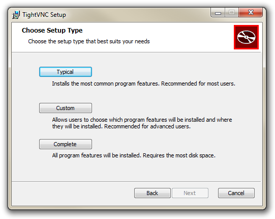
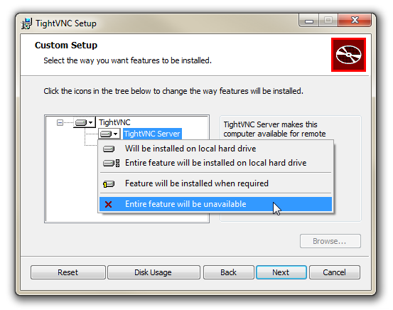
We only want to install the viewer for the software (since we don’t want to make our Windows desktop available to other computers on the network). So click on ‘Custom’ and then click on the ‘TightVNC Server’ drop-down and select ‘Entire feature will be unavailable’. This will prevent the server side of the software being installed on our machine (thanks to Graham Travener for the hint to disable this), then select ‘Next’.
The ‘Select Additional Tasks’ selections can be left at their defaults.
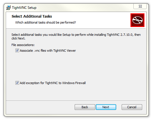
Then click on ‘Install’.
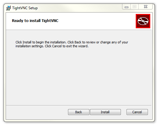
Click on ‘Finish’ after a short install period and you should be done. You can now find ‘TightVNC Viewer’ from the start menu (but don’t bother running it yet as we still need to set up the Raspberry Pi!).
Setting up the Server (Raspberry Pi)
We’ll approach the process of installing the TightVNC server on the Raspberry Pi in two stages. In the first stage we’ll install the software, run it and test it. In the second stage we’ll configure it so that it starts automatically when the Raspberry Pi boots up which means that we can work remotely from that point.
Installing software on the Raspberry Pi is a pretty easy task. All you need to do is from the command line, type;
You will recall that the sudo portion of the command makes sure that you will have the correct permissions (in this case to run a command). The command that is run is one of the family of apt-get commands, which deal with package management. The install part of the command tells the apt-get program to not just get the software, but to install it as well. Lastly, tightvncserver is the application that will be installed. For more information on the apt-get command, see the Glossary.
The Raspberry Pi may ask you if you want to continue once it’s done some checks that it can get the software (and any other software that it might be dependant on). Just answer ‘y’ if prompted.
After a short scrolling of messages, tightvncserver should be installed!
Now we can run the program by typing in;
You will be prompted to enter a password that we will use on our Windows client software to authenticate that we are the right people connecting. Feel free to enter an appropriate password (believe it or not in this crazy security conscious world, there is a maximum length of password of 8 characters).
You will be asked if you want to have a ‘view-only’ password that would allow a client to look at, but not interact with the remote desktop (in this case I wouldn’t bother).
The software will then assign us a desktop and print out a couple of messages. One that we will need to note will say something like;
New 'X' desktop is raspberrypi:1
The :1 informs us of the number of the desktop session that we will be looking at (since you can have more than one).
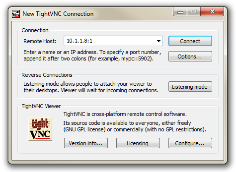
Now on the Windows desktop, start the TightVNC Viewer program. We will see a dialogue box asking which remote host we want to connect to. In this box we will put the IP address of our Raspberry Pi followed by a colon (:) and the number of the desktop that was allocated in the tightvncserver program (10.1.1.8:1).
We will be prompted for the password that we set to access the remote desktop;
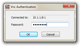
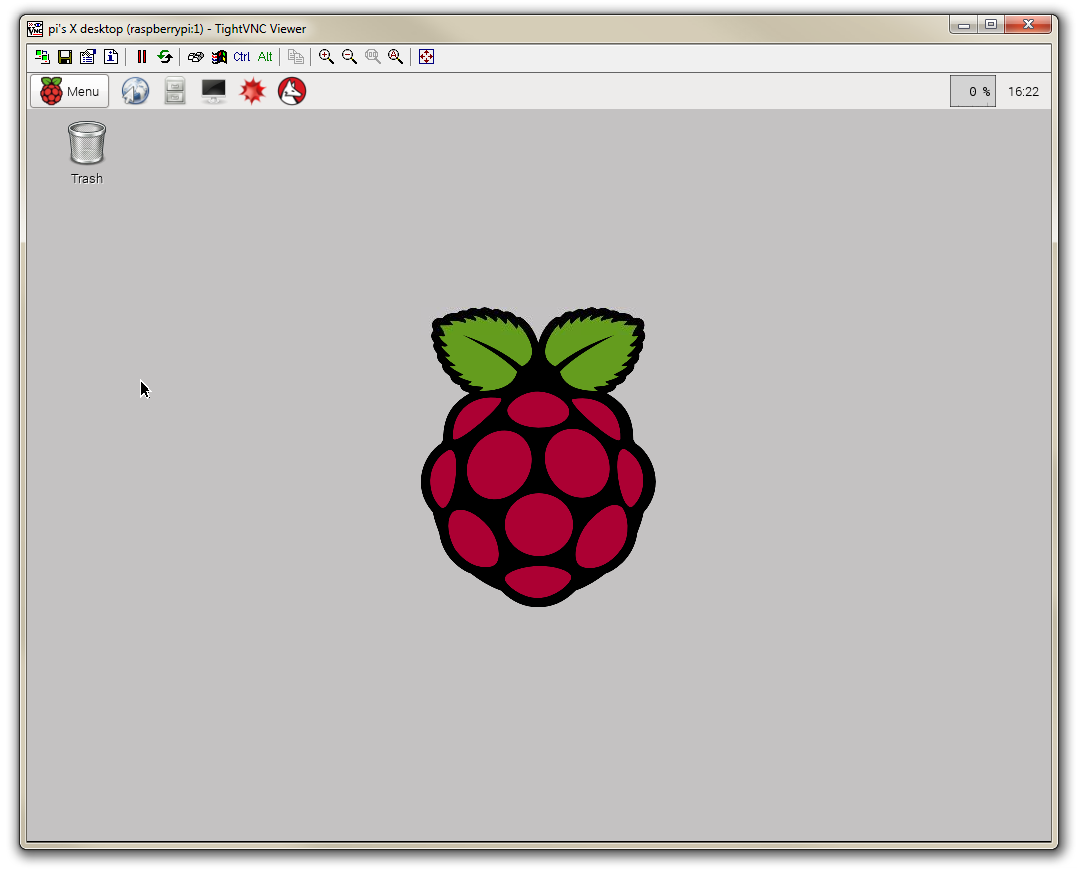
In theory we will then be connected to a remote desktop view of the Raspberry Pi from our Windows desktop.
Take a moment to interact with the connection and confirm that everything is working as anticipated.
Copying and Pasting between Windows and the Raspberry Pi
Remotely accessing the Raspberry Pi is a great thing to be able to to, but to make the experience even more useful we need to have the ability to copy and paste between the Windows environment and the Raspberry Pi.
We can certainly survive without this feature, but being able to carry out research on a more powerful machine and then copy-paste code from one to the other is a real advantage.
On the raspberry Pi, first we have to install ‘autocutsel’ as follows;
Then we need to edit the ‘xstartup’ file as follows;
… and add in the line autocutsel -fork to start it when the graphical display starts;
#!/bin/sh

xrdb $HOME/.Xresources
xsetroot -solid grey
autocutsel -fork
#x-terminal-emulator -geometry 80x24+10+10 -ls -title "$VNCDESKTOP Desktop" &
#x-window-manager &
# Fix to make GNOME work
export XKL_XMODMAP_DISABLE=1
/etc/X11/Xsession
Make sure that you place the autocutsel -fork in the position indicated in the example above as otherwise it will not work as desired.
All that remains is to reboot the Raspberry Pi for the changes to take effect.
Starting TightVNC at boot on the Pi.
Having a remote desktop is extremely useful, but if we need to run the tightvncserver program on the Raspberry Pi each time we want to use the remote desktop, it would be extremely inconvenient. What we will do instead is set up tightvncserver so that it starts automatically each time the Raspberry Pi boots up.
To do this we are going to use a little bit of Linux cleverness. We’ll explain it as we go along, but be aware, some will find the explanations a little tiresome (if you’re already familiar) but I’m sure that there will be some readers who will benefit.
Our first task will be to edit the file /etc/rc.local. This file can contain commands that get run on start-up. If we look at the file we can see that there is already few entries in there;
#!/bin/sh -e
#
# rc.local
#
# This script is executed at the end of each multiuser runlevel.
# Make sure that the script will "exit 0" on success or any other
# value on error.
#
# In order to enable or disable this script just change the execution
# bits.
#
# By default this script does nothing.

# Print the IP address
_IP=$(hostname -I) || true
if [ "$_IP" ]; then
  printf "My IP address is %s\n" "$_IP"
fi

exit 0
The first set of lines with a hash mark (#) in front of them are comments. These are just there to explain what is going on to someone reading the file.
The lines of code towards the bottom clearly have something to do with the IP address of the computer. In fact they are a short script that checks to see if the Raspberry Pi has an IP address and if it does, it prints it out. If you recall when we were setting out IP address earlier in the chapter, we could see the IP address printed out on the screen when the Pi booted up like so
My IP address is 10.1.1.8

Raspbian GNU/Linux 7 raspberrypi tty1

raspberrypi login:
This piece of script in rc.local is the code responsible for printing out the IP address!
We will add the following command into rc.local;
su - pi -c '/usr/bin/tightvncserver :1'
This command switches user to be the ‘pi’ user with su - pi. The su stands for ‘switch user’ the dash (-) makes sure that the user pi’s environment (like all their settings) are used correctly and pi is the user.
The -c option declares that the next piece of the line is going to be the command that will be run and the part inside the quote marks ('/usr/bin/tightvncserver :1') is the command.
The command in this case executes the file tightvncserver which is in the /usr/bin directory and it specifies that we should start desktop session 1 (:1).
To do this we will edit the rc.local file with the following command;
Add in our lines so that the file looks like the following;
#!/bin/sh -e
#
# rc.local
#
# This script is executed at the end of each multiuser runlevel.
# Make sure that the script will "exit 0" on success or any other
# value on error.
#
# In order to enable or disable this script just change the execution
# bits.
#
# By default this script does nothing.

# Print the IP address
_IP=$(hostname -I) || true
if [ "$_IP" ]; then
  printf "My IP address is %s\n" "$_IP"
fi

# Start tightvncserver
su - pi -c '/usr/bin/tightvncserver :1'

exit 0
(We can also add our own comment into the file to let future readers know what’s going on)
That should be it. We should now be able to test that the service starts when the Pi boots by typing in;
When the Raspberry has finished starting up again, we should be able to see in the list of text that shows up while the boot sequence is starting the line New 'X' desktop is raspberrypi:1.
Assuming that this is the case, we can now start the TightVNC Viewer program on the Windows desktop and we will be able to see a remote view of the Raspberry Pi’s desktop.
Now for the big test.
Power off the Raspberry Pi;
Now physically turn off the power to the Pi.
Unplug the keyboard / mouse and the video from the unit so that there is only the power connector and the network cable left plugged in.
Now turn the power back on.
(We will need to wait for 30 seconds or so while it boots up)
Start the TightVNC Viewer program on the Windows desktop and we will be able to see a remote view of the Raspberry Pi’s desktop but this time the Pi doesn’t have a keyboard / mouse or video screen attached.
If this is the first time that you’ve done something like this it can be a very liberating feeling. Suddenly you can see possibilities for using the Raspberry Pi that do not involve having it physically tethered to a lot of extra peripherals. And if you’re anyone like me, the next thing you do is ask yourself, “How can I get rid of that network cable?”.
Remote access via SSH
Secure Shell (SSH) is a network protocol that allows secure data communication, remote command-line login, remote command execution, and other secure network services between two networked computers. It connects, via a secure channel over an insecure network, a server and a client running SSH server and SSH client programs, respectively (there’s the client-server model again).
In our case the SSH program on the server is running sshd and on the Windows machine we will use a program called ‘PuTTY’.
Setting up the Server (Raspberry Pi)
This is definitely one of the easiest set-up steps since SSH is already installed on Raspbian.
To check that it is there and working type the following from the command line;
The Pi should respond with the message that the program sshd is running.

Installing SSH on the Raspberry Pi.
If for some reason SSH is not installed on your Pi, you can easily install with the command;
Once this has been done SSH will start automatically when the Raspberry Pi boots up.
Setting up the Client (Windows)
The client software we will use is called ‘Putty’. It is open source and available for download from here.
On the download page there are a range of options available for use. The best option for us is most likely under the ‘For Windows on Intel x86’ heading and we should just download the ‘putty.exe’ program.
Save the file somewhere logical as it is a stand-alone program that will run when you double click on it (you can make life easier by placing a short-cut on the desktop).
Once we have the file saved, run the program by double clicking on it and it will start without problem.
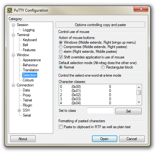
The first thing we will set-up for our connection is the way that the program recognises how the mouse works. In the ‘Window’ Category on the left of the PuTTY Configuration box, click on the ‘Selection’ option. On this page we want to change the ‘Action of mouse’ option from the default of ‘Compromise (Middle extends, Right paste)’ to ‘Windows (Middle extends, Right brings up menu)’. This keeps the standard Windows mouse actions the same when you use PuTTY.
Now select the ‘Session’ Category on the left hand menu. Here we want to enter our static IP address that we set up earlier (10.1.1.8 in the example that we have been following, but use your one) and because we would like to access this connection on a frequent basis we can enter a name for it as a saved session (In the scree-shot below it is imaginatively called ‘Raspberry Pi’). Then click on ‘Save’.
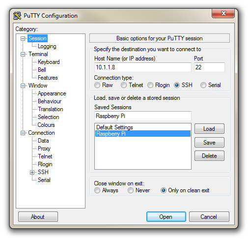
Now we can select our raspberry Pi Session (per the screen-shot above) and click on the ‘Open’ button.
The first thing you will be greeted with is a window asking if you trust the host that you’re trying to connect to.
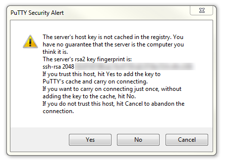
In this case it is a pretty safe bet to click on the ‘Yes’ button to confirm that we know and trust the connection.
Once this is done, a new terminal window will be shown with a prompt to login as: . Here we can enter our user name (‘pi’) and then our password (if it’s still the default it is ‘raspberry’).
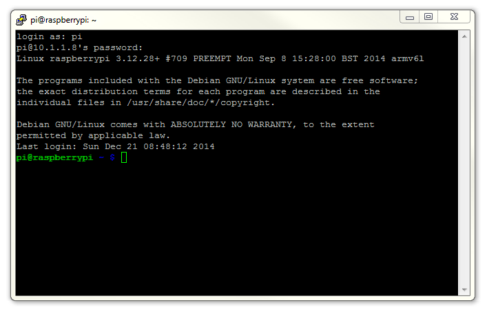
There you have it. A command line connection via SSH. Well done.
As I mentioned at the end of the section on remotely accessing the Raspberry Pi’s GUI, if this is the first time that you’ve done something like this it can be a very liberating feeling. To complete the feeling of freedom let’s set up a wireless network connection.
Setting up a WiFi Network Connection
Our set-up of the Raspberry Pi has us at a point where we are able to carry out all the (computer interface) interactions we will require via a remote desktop. However, the Raspberry Pi is making that remote connection via a fixed network cable. It could be argued that to fulfil the ultimate aspirations of sensing different aspects of our world we will need to be able to place the platform that we want to do the measuring in a position where we have no physical network connection. The most obvious solution to this conundrum is to enable a wireless connection.
It should be noted that enabling a wireless network will not be a requirement for everyone and as such, I would only recommend it if you need to. It means that you will need to purchase a USB WiFi dongle and correctly configure it which as it turns out can be something of an exercise. In my own experience, I found that choosing the right wireless adapter was the key to making the job simple enough to be able to recommend it to new comers. Not all WiFi adapters are well supported and if you are unfamiliar with the process of installing drivers or compiling code, then I would recommend that you opt for an adapter that is supported and will work ‘out of the box’. There is an excellent page on elinux.org which lists different adapters and their requirements. I eventually opted for the Edimax EW-7811Un which literally ‘just worked’ and I would recommend it to others for it’s ease of use and relatively low cost (approximately $15 US).

To install the wireless adapter we should start with the Pi powered off and install it into a convenient USB connection. When we turn the power on we will see the normal range of messages scroll by, but if we’re observant we will note that there are a few additional lines concerning a USB device. These lines will most likely scroll past, but once the device has finished powering up and we have logged in we can type in…
… which will show us a range of messages about drivers that are loaded to support discovered hardware.
Towards the end of the list (it shouldn’t have scrolled off the window) will be a series of messages that describe the USB connectors and what is connected to them. In particular we could see a group that looks a little like the following;
[3.382731] usb 1-1.2: new high-speed USB device number 4 using dwc_otg
[3.494250] usb 1-1.2: New USB device found, idVendor=7392, idProduct=7811
[3.507749] usb 1-1.2: New USB device strings: Mfr=1, Product=2, SerialNumber=3
[3.520230] usb 1-1.2: Product: 802.11n WLAN Adapter
[3.542690] usb 1-1.2: Manufacturer: Realtek
[3.560641] usb 1-1.2: SerialNumber: 00345767831a5e
That is our USB adapter which is plugged into USB slot 2 (which is the ‘2’ in usb 1-1.2:). The manufacturer is listed as ‘Realtek’ as this is the manufacturer of the chip-set in the adapter that Edimax uses.
In the same way that we edited the /etc/network/interfaces file earlier to set up the static IP address we will now edit it again with the command…
This time we will edit the interfaces file so that it looks like the following;
auto lo

iface lo inet loopback
iface eth0 inet dhcp

allow-hotplug wlan0
auto wlan

iface wlan0 inet static
  address 10.1.1.8
  netmask 255.255.255.0
  gateway 10.1.1.1
  wpa-ssid "homenetwork"
  wpa-psk "h0mepassw0rd"
Here we have reverted the eth0 interface (the wired network connection) to have it’s network connection assigned dynamically (iface eth0 inet dhcp).
Our wireless lan (wlan0) is now designated to be a static IP address (with the details that we had previously assigned to our wired connection) and we have added the ‘ssid’ (the network name) of the network that we are going to connect to and the password for the network. Save the file.
To allow the changes to become operative we can type in;
Once we have rebooted, we can check the status of our network interfaces by typing in;
This will display the configuration for our wired Ethernet port, our ‘Local Loopback’ (which is a fancy way of saying a network connection for the machine that you’re using, that doesn’t require an actual network (ignore it in the mean time)) and the wlan0 connection which should look a little like this;
wlan0 Link encap:Ethernet HWaddr 80:1f:02:f4:21:85
      inet addr:10.1.1.8 Bcast:10.1.1.255 Mask:255.255.255.0
      UP BROADCAST RUNNING MULTICAST MTU:1500 Metric:1
      RX packets:213 errors:0 dropped:90 overruns:0 frame:0
      TX packets:54 errors:0 dropped:0 overruns:0 carrier:0
      collisions:0 txqueuelen:1000
      RX bytes:88729 (86.6 KiB) TX bytes:6467 (6.3 KiB)
This would indicate that our wireless connection has been assigned the static address that we were looking for (10.1.1.8).
We should be able to test our connection by connecting to the Pi via the TightVNC Viewer on the Windows desktop.
In theory you are now the proud owner of a computer that can be operated entirely separate from all connections except power.
Web Server and PHP
Because we want to be able to explore the data we will be collecting, we need to set up a web server that will present web pages to other computers that will be browsing within the network (remembering that this is not intended to be connected to the internet, just inside your home network). At the same time as setting up a web server on the Pi we will install PHP.
At the command line run the following command;
We’re familiar with apt-get already, but this time we’re including more than one package in the installation process. Specifically we’re including apache2, php5 and libapache2-mod-php5.
‘apache2’ is the name of the web server and php5, libapache2-mod-php5 are for PHP.
The Raspberry Pi will advise you of the range of additional packages that will be installed at the same time (to support those we’re installing (these additional packages are dependencies)). Agree to continue and the installation will proceed. This should take a few minutes or more (depending on the speed of your Internet connection).
Once complete we need to restart our web server with the following command;
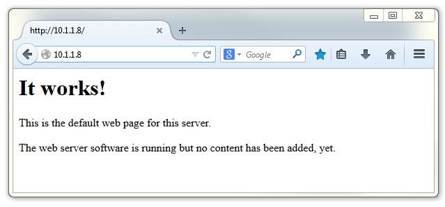
We can now test our web server from the windows desktop machine.
Open up a web browser and type in the IP address of the Raspberry Pi into the URL bar at the top. Hopefully we will see…
We could also test the web server from the Pi itself. From the Raspberry Pi’s desktop start the Epiphany Web Browser and enter either 10.1.1.8 (or 127.0.1.1 which is the address that the Pi can ‘see’ internally (called the ‘localhost’ address)) into the URL bar at the top. We should see the following…
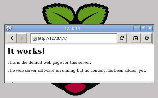
Congratulations! We have a web server.
Tweak permissions for easier web file editing
The default installation of the Apache web server has the location of the files that make up our web server owned by the ‘root’ user. This means that if we want to edit them we need to do so with the permissions of the root user. This can be easily achieved by typing something like sudo nano /var/www/index.html, but if we want to be able to use an editor from our GUI desktop, we will need the permissions to be set to allow the ‘pi’ user to edit them without having to invoke sudo.
We’re going to do this by making a separate group (‘www-data’ will be its name) the owners of the /var/www directory (where our web files will live) then we will add the ‘pi’ user to the ‘www-data’ group.
We start by making the ‘www-data’ group and user the owner of the /var/www directory with the following command;
(For more information on the chown command check out the Glossary)
Then we allow the ‘www-data’ group permission to write to the directory;
(For more information on the chmod command check out the Glossary)
Then we add the ‘pi’ user to the ‘www-data’group;
(For more information on the usermod command check out the Glossary)
This change in permissions are best enacted by rebooting the Raspberry Pi;
Now the ‘pi’ user has the ability to edit files in the /var/www directory without problem.
Database
As mentioned earlier in the book, we will use a MySQL database to store the information that we collect.
We will install MySQL in a couple of steps and then we will install the database administration tool phpMyAdmin to make our lives easier.
MySQL
From the command line run the following command;
The Raspberry Pi will advise you of the range of additional packages that will be installed at the same time. Agree to continue and the installation will proceed. This should take a few minutes or more (depending on the speed of your internet connection).
You will be prompted (twice) to enter a root password for your database. Note it down somewhere safe;
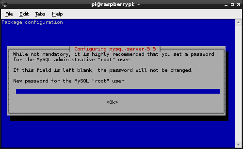
Make this a reasonably good password. You won’t need it too much, so it’s reasonable to make it more secure.
Once this installation is complete, we will install a couple more packages that we will use in the future when we integrate PHP and Python with MySQL. To do this enter the following from the command line;
Agree to the installed packages and the installation will proceed fairly quickly.
That’s it! MySQL server installed. However, it’s not configured for use, so we will install phpMyAdmin to help us out.
phpMyAdmin
phpMyAdmin is free software written in PHP to carry out administration of a MySQL database installation.
To begin installation run the following from the command line;
Agree to the installed packages and the installation will proceed.
You will receive a prompt to ask what sort of web server we are using;
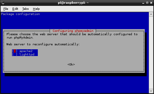
Select ‘apache2’ and tab to ‘Ok’ to continue.
We will then be prompted to configure the database for use with phpMyAdmin;
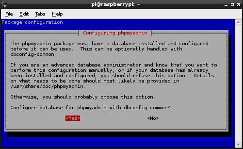
We want the program to look after it for us, so select ‘Yes’ and continue.
We will then be prompted for the password for the administrative account for the MySQL database.
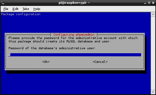
This is the root password for MySQL that we set up earlier. Enter it and tab to ‘Ok’ to continue.
We will then be prompted for a password for phpMyAdmin to access MySQL.
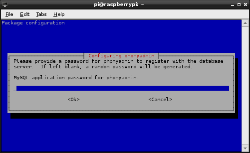
I have used the same password as the MySQL root password in the past to save confusion, but over to you. Just make sure you note it down :-). Then tab to ‘Ok’ to continue (and confirm).
The installation should conclude soon.
Once finished, we need to edit the Apache web server configuration to access phpMyAdmin. To do this execute the following command from the command line;
Get to the bottom of the file by pressing ctrl-v a few times and there we want to add the line;
Include /etc/phpmyadmin/apache.conf
Save the file and then restart Apache2;
This should have everything running.
Now if we go to our browser on the Windows (or on the Raspberry Pi) desktop and enter the IP address followed by /phpmyadmin (in the case of our example 10.1.1.8/phpmyadmin) it should start up phpMyAdmin in the browser.
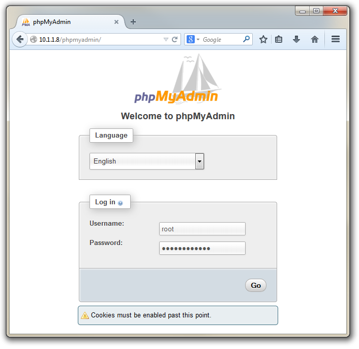
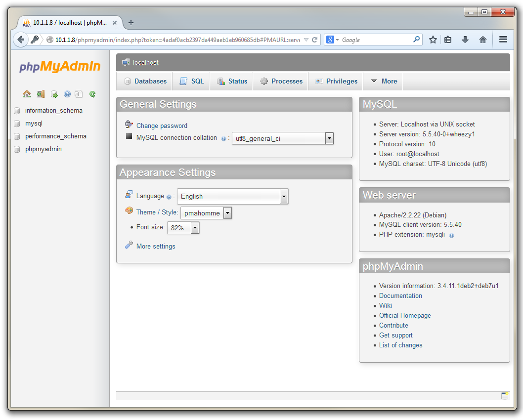
If you enter the username as ‘root’ and the MySQL root password that we set earlier, it will open up the phpMyAdmin interface.
Allow access to the database remotely
It might seem a little strange to say that we want to allow access to the database remotely since this would appear to be part of the grand plan all along. But there are different types of access and in particular there may be a need for a remote computer to access the database directly.
This direct access occurs when (for example) a web server on a different computer to the Raspberry Pi wants to use the data. In this situation it would need to request access to the database over the network by referencing the host computer that the database was on (in this case we have specified that it is on the computer at the IP address 10.1.1.8).
By default the Raspberry Pi’s Operating System is set up to deny that access and if this is something that you want to allow this is what you will need to do.
On the Raspberry Pi we need to edit the configuration file ‘my.cnf’ in the directory /etc/mysql/. We do this with the following command;
Scroll down the file a short way till we find the section [mysqld]. Here we need to edit the line that reads something similar to;
bind-address = 127.0.0.1
This line is telling MySQL to only listen to commands that come from the ‘localhost’ network (127.0.0.1). Essentially only the Raspberry Pi itself. We can change this by inserting a ‘#’ in front of the line which will turn the line into a comment instead of a configuration option. So change it to look like this;
# bind-address = 127.0.0.1
Once we have saved the file, we need to restart the MySQL service with the following command;
Create users for the database
Our database has an administrative (root) user, but for our future purposes, we will want to add a couple more users to manage the security of the database in a responsible way.
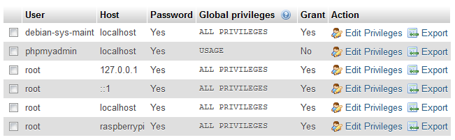
If we click on the ‘Privileges’ tab in phpMyAdmin we can see the range of users that are already set up.
We will create an additional two users. One that can only read (select) data from our database and another that can put data into (insert) the database. Keeping these functions separate gives us some flexibility in how we share the data in the future. For example we could be reasonably comfortable providing the username and password to allow reading the data to a wide range of people, but we should really only allow our future scripts the ability to insert data into the database.
From the ‘Privileges’ tab, select ‘Add a new user’;
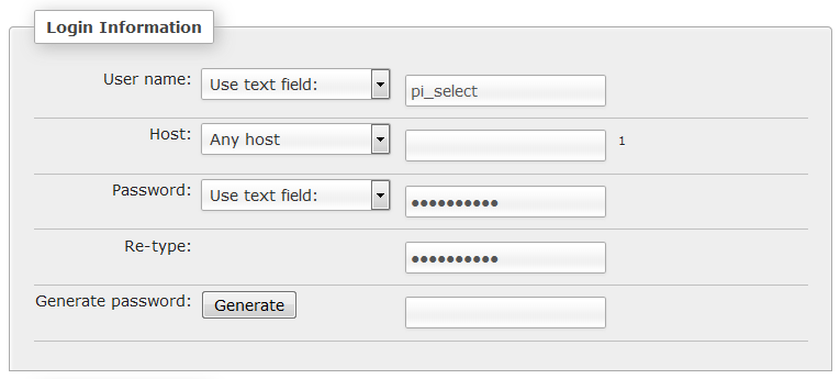
Enter a user name and password.
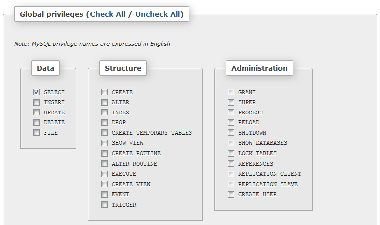
Then we scroll down a little and select the type of access we want the pi_select user to have in the ‘Global privileges’ section. For the pi_select user under ‘Data’ we want to tick ‘SELECT’.
Then press the ‘Create User’ button and we’ve created a user.
For the second user with the ability to insert data (let’s call the user ‘pi_insert’), go through the same process, but tick the ‘SELECT’ and the ‘INSERT’ options for the data.
When complete we should be able to see that both of our users look similar to the following;

Create a database
When we read data from our sensors, we will record them in a database. MySQL is a database program, but we still need to set up a database inside that program. In fact while we will set up a database in this step, when we come to record and explore our data we will be dealing with a ‘table’ of data that will exist inside a database.
For the purposes of getting ourselves set up we need to create a database. If we go to the ‘Databases’ tab we can enter a name for a new database (here I’ve called one ‘measurements’) and click on ‘Create’.
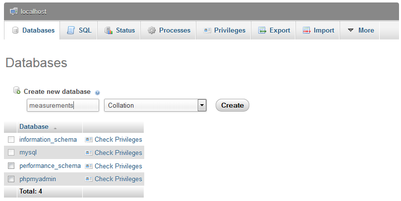
Congratulations! We’re set up and ready to go.
Backup the Configured SD Card
Once we have installed our base of software it is a good idea to copy an image of the SD card onto the Windows machine so that we can recreate (clone) the installation back to the current state.
We will use the Open Source utility Win32DiskImager again. Use the SD card reader capable of accepting your micro SD card and note the drive letter of the SD card.
Start the Win32 Disk Imager program.
Select the correct drive letter for your SD card (make sure it’s the right one) and enter a new name and location for our new Raspbian disk image. Then select ‘Read’ and the disk imager will read the image from the SD card and create a new disk image on the windows machine at the location you have specified.
Once the process is finished, exit the disk imager and eject the card from the computer and you’re done.
Exploring data with a simple line graph
As explained earlier in the chapter, our aim is to present the data we are recording in a form that will make it easy to interpret and digest. What is presented in this portion of the set-up of the Raspberry Pi is not required to get up and going. Instead it is a description of a simple visualisation technique that will probably be applicable for just about any measured value over time. This is also the code for the first project that we will examine (measuring a single temperature).
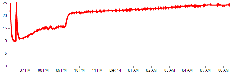
To achieve this aim a simple mechanism to show data changing over time is a line graph. To do this we will build a web page that our web server will host that will look at the data in a table on our database and show it using a combination of PHP, HTML, JavaScript and d3.js.
Ultimately we’re going to aim for a simple line graph that will look a little like this (except the data will be different of course);
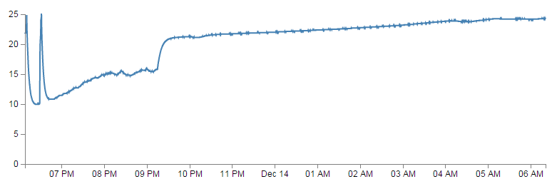
You would be well within your rights to wonder if ‘That’s it?’. But think of this simple graph as the foot into the door of presenting data automatically and dynamically. We will explore different techniques for showing data as we measure different things and hopefully learn a little more about visualizing information as we go. In the mean time, the sum of all our efforts is a simple line graph :-).
The full code
The code for this web page may look slightly intimidating at first glance, but we will step through it and explain what we have and it can form the basis for displaying a range of the data that we collect.
The full code will be named s_temp.php and will be saved in the /var/www directory. The full script (which in this case is for the single temperature measurement) is as follows;
<?php
$hostname = 'localhost';
$username = 'pi_select';
$password = 'xxxxxxxxxx';

try {
    $dbh = new PDO("mysql:host=$hostname;dbname=measurements", $username, $pa\
ssword);

    /*** The SQL SELECT statement ***/
    $sth = $dbh->prepare("
       SELECT  `dtg`, `temperature` FROM  `temperature`
    ");
    $sth->execute();

    /* Fetch all of the remaining rows in the result set */
    $result = $sth->fetchAll(PDO::FETCH_ASSOC);

    /*** close the database connection ***/
    $dbh = null;

}
catch(PDOException $e)
    {
        echo $e->getMessage();
    }

$json_data = json_encode($result);
?>
<!DOCTYPE html>
<meta charset="utf-8">
<style> /* set the CSS */
body { font: 12px Arial;}
path {
stroke: steelblue;
stroke-width: 2;
fill: none;
}
.axis path,
.axis line {
fill: none;
stroke: grey;
stroke-width: 1;
shape-rendering: crispEdges;
}
</style>
<body>
<!-- load the d3.js library -->
<script src="http://d3js.org/d3.v3.min.js"></script>
<script>
// Set the dimensions of the canvas / graph
var margin = {top: 30, right: 20, bottom: 30, left: 50},
width = 800 - margin.left - margin.right,
height = 270 - margin.top - margin.bottom;
// Parse the date / time
var parseDate = d3.time.format("%Y-%m-%d %H:%M:%S").parse;
// Set the ranges
var x = d3.time.scale().range([0, width]);
var y = d3.scale.linear().range([height, 0]);
// Define the axes
var xAxis = d3.svg.axis().scale(x)
.orient("bottom");
var yAxis = d3.svg.axis().scale(y)
.orient("left").ticks(5);
// Define the line
var valueline = d3.svg.line()
.x(function(d) { return x(d.dtg); })
.y(function(d) { return y(d.temperature); });
// Adds the svg canvas
var svg = d3.select("body")
.append("svg")
.attr("width", width + margin.left + margin.right)
.attr("height", height + margin.top + margin.bottom)
.append("g")
.attr("transform",
"translate(" + margin.left + "," + margin.top + ")");
// Get the data
<?php echo "data=".$json_data.";" ?>
data.forEach(function(d) {
d.dtg = parseDate(d.dtg);
d.temperature = +d.temperature;
});
// Scale the range of the data
x.domain(d3.extent(data, function(d) { return d.dtg; }));
y.domain([0, d3.max(data, function(d) { return d.temperature; })]);
// Add the valueline path.
svg.append("path")
.attr("d", valueline(data));
// Add the X Axis
svg.append("g")
.attr("class", "x axis")
.attr("transform", "translate(0," + height + ")")
.call(xAxis);
// Add the Y Axis
svg.append("g")
.attr("class", "y axis")
.call(yAxis);
</script>
</body>
The code is roughly in three blocks. The first block is the PHP section at the start of the script. This is everything between the <?php and ?> instances. The second is an HTML section between <!DOCTYPE html> and </body>. The third is actually contained within the second section and is the code between <script> and </script>.
PHP
The job of our block of PHP at the start of the file is to select the data that we want from our database and to store it in a variable that we will then use later in the code.
The cool thing about PHP is that when it runs, it runs on the server where the file exists (in this case the Raspberry Pi). This means that that entire block is essentially invisible to a remote user just wanting to view the graph (if they chose to look at the code that drew the graph). That’s a good thing, because you will notice that we have our password in the file and broadcasting passwords to the world (in spite of the fact that this is never intended to go outside a home network) is not really a good thing. More alert readers will pick up that we are using a technique for querying the database called PDO. This is a newer method for accessing a MySQL (and other types) database and is a more secure method than the traditional method (which early readers of this book would have seen).
The other thing that observant readers will notice is that we actually have two pieces of PHP code in the file. The large block at the start and a smaller snippet in the middle of the HTML and JavaScript (<?php echo "data=".$json_data.";" ?>). We’ll cover the second snippet when we talk about the JavaScript portion as by then it will be a lot more obvious what we’re trying to do.
The code
The section of code we will explain first is as follows;
<?php
$hostname = 'localhost';
$username = 'pi_select';
$password = 'xxxxxxxxxx';

try {
    $dbh = new PDO("mysql:host=$hostname;dbname=measurements",
                               $username, $password);

    /*** The SQL SELECT statement ***/
    $sth = $dbh->prepare("
       SELECT  `dtg`, `temperature` FROM  `temperature`
    ");
    $sth->execute();

    /* Fetch all of the remaining rows in the result set */
    $result = $sth->fetchAll(PDO::FETCH_ASSOC);

    /*** close the database connection ***/
    $dbh = null;

}
catch(PDOException $e)
    {
        echo $e->getMessage();
    }

$json_data = json_encode($result);
?>
The <?php line at the start and the ?> line at the end form the wrappers that allow the requesting page to recognise the contents as PHP and to execute the code rather than downloading it for display.
The following lines set up a range of important variables;
$hostname = 'localhost';
$username = 'pi_select';
$password = 'xxxxxxxxxx';
Hopefully you will recognise that these are the configuration details for the MySQL database that we set up. There’s the user and the password (remember, the script isn’t returned to the browser, the browser doesn’t get to see the password and in this case our user has a very limited set of privileges). There’s the host address that contains our database (in this case it’s local (on the same server), so we use localhost, but if the database was on a remote server, we would just include its address (10.1.1.8 in our example)) and there’s the database we’re going to access.
Then we use those variables to define how we will connect to the server and the database…
    $dbh = new PDO("mysql:host=$hostname;dbname=measurements",
                               $username, $password);
… then we prepare our query that will request the data from the database table…
    $sth = $dbh->prepare("
       SELECT  `dtg`, `temperature` FROM  `temperature`
    ");
(This particular query is telling the database to SELECT our date/time data (from the dtg column) and the temperature values (from the temperature column) FROM the table temperature.)
… and execute the query.
$sth->execute();
We fetch all the returned data and place it in an associative array.
$result = $sth->fetchAll(PDO::FETCH_ASSOC);
Then we close the connection to the database.
$dbh = null;
…and then we check to see if it was successful. If it wasn’t, we output the exception message with our catch section;
catch(PDOException $e)
    {
        echo $e->getMessage();
    }
We then encode the contents of our array in a the JSON format (follow the link for a section in the appendices that explains how JSON works).
$json_data = json_encode($result);
Whew!
HTML
This stands for HyperText Markup Language and is the stuff that web pages are made of. Check out the definition and other information on Wikipedia for a great overview. Just remember that all we’re going to use HTML for is to hold the code that we will use to present our information.
The HTML code we are going to examine also includes Cascading Style Sheets (everyone appears to call them ‘Style Sheets’ or ‘CSS’) which are a language used to describe the formatting (or “look and feel”) of a document written in a markup language (HTML in this case). The job of CSS is to make the presentation of the components we will draw with D3 simpler by assigning specific styles to specific objects. One of the cool things about CSS is that it is an enormously flexible and efficient method for making everything on the screen look more consistent and when you want to change the format of something you can just change the CSS component and the whole look and feel of your graphics will change.
Here’s the HTML portions of the code;
<!DOCTYPE html>
<meta charset="utf-8">
<style>

    The CSS is in here

</style>
<body>
<script src="http://d3js.org/d3.v3.min.js"></script>

<script>

    The D3 JavaScript code is here

</script>
</body>
Compare it with the full code. It kind of looks like a wrapper for the CSS and JavaScript. You can see that it really doesn’t boil down to much at all (that doesn’t mean it’s not important).
There are plenty of good options for adding additional HTML stuff into this very basic part for the file, but for what we’re going to be doing, we really don’t need to bother too much.
One thing probably worth mentioning is the line;
<script src="http://d3js.org/d3.v3.min.js"></script>
That’s the line that identifies the file that needs to be loaded to get D3 up and running. In this case the file is sourced from the official d3.js repository on the internet (that way we are using the most up to date version). The D3 file is actually called d3.v3.min.js which may come as a bit of a surprise. That tells us that this is version 3 of the d3.js file (the v3 part) which is an indication that it is separate from the v2 release, which was superseded in late 2012. The other point to note is that this version of d3.js is the minimised version (hence min). This means that any extraneous information has been removed from the file to make it quicker to load.
The two parts that we left out are the CSS and the D3 JavaScript.
CSS
The CSS is as follows;
body { font: 12px Arial;}

path {
    stroke: steelblue;
    stroke-width: 2;
    fill: none;
}

.axis path,
.axis line {
    fill: none;
    stroke: grey;
    stroke-width: 1;
    shape-rendering: crispEdges;
}
Cascading Style Sheets give you control over the look / feel / presentation of web content. The idea is to define a set of properties to objects in the web page.
They are made up of ‘rules’. Each rule has a ‘selector’ and a ‘declaration’ and each declaration has a property and a value (or a group of properties and values).
For instance in the example code for this web page we have the following rule;
body { font: 12px Arial;}
body is the selector. This tells you that on the web page, this rule will apply to the ‘body’ of the page. This actually applies to all the portions of the web page that are contained in the ‘body’ portion of the HTML code (everything between <body> and </body> in the HTML bit).
{ font: 12px Arial;} is the declaration portion of the rule. It only has the one declaration which is the bit that is in between the curly braces.
So font: 12px Arial; is the declaration. The property is font: and the value is 12px Arial;. This tells the web page that the font that appears in the body of the web page will be in 12 px Arial.
What about the bit that’s like;
path {
    stroke: steelblue;
    stroke-width: 2;
    fill: none;
}
Well, the whole thing is one rule, ‘path’ is the selector. In this case, ‘path’ is referring to a line in the D3 drawing nomenclature.
For that selector there are three declarations. They give values for the properties of ‘stroke’ (in this case colour), ‘stroke-width’ (the width of the line) and ‘fill’ (we can fill a path with a block of colour).
We could test the changes by editing our file to show a thicker line in a different colour as so;
path {
    stroke: red;
    stroke-width: 4;
    fill: none;
}
By all means have a play with the settings and see what the end result is.
JavaScript and d3.js
JavaScript is what’s called a ‘scripting language’. It is the code that will be contained inside the HTML file that will make D3 do all its fanciness. In fact, D3 is a JavaScript Library. JavaScript is the language D3 is written in.
Knowing a little bit about this would be really good, but to be perfectly honest, I didn’t know anything about it before I started writing ‘D3 Tips and Tricks’. I read a book along the way (JavaScript: The Missing Manual from O’Reilly) and that helped with context, but the examples that are available for D3 graphics are understandable, and with a bit of trial and error, you can figure out what’s going on.
The D3 JavaScript part of the code is as follows;
// Set the dimensions of the canvas / graph
var margin = {top: 30, right: 20, bottom: 30, left: 50},
    width = 800 - margin.left - margin.right,
    height = 270 - margin.top - margin.bottom;

// Parse the date / time
var parseDate = d3.time.format("%Y-%m-%d %H:%M:%S").parse;

// Set the ranges
var x = d3.time.scale().range([0, width]);
var y = d3.scale.linear().range([height, 0]);

// Define the axes
var xAxis = d3.svg.axis().scale(x)
    .orient("bottom");

var yAxis = d3.svg.axis().scale(y)
    .orient("left").ticks(5);

// Define the line
var valueline = d3.svg.line()
    .x(function(d) { return x(d.dtg); })
    .y(function(d) { return y(d.temperature); });

// Adds the svg canvas
var svg = d3.select("body")
    .append("svg")
        .attr("width", width + margin.left + margin.right)
        .attr("height", height + margin.top + margin.bottom)
    .append("g")
        .attr("transform",
              "translate(" + margin.left + "," + margin.top + ")");

// Get the data
<?php echo "data=".$json_data.";" ?>
data.forEach(function(d) {
	d.dtg = parseDate(d.dtg);
	d.temperature = +d.temperature;
});

// Scale the range of the data
x.domain(d3.extent(data, function(d) { return d.dtg; }));
y.domain([0, d3.max(data, function(d) { return d.temperature; })]);

// Add the valueline path.
svg.append("path")
	.attr("d", valueline(data));

// Add the X Axis
svg.append("g")
	.attr("class", "x axis")
	.attr("transform", "translate(0," + height + ")")
	.call(xAxis);

// Add the Y Axis
svg.append("g")
	.attr("class", "y axis")
	.call(yAxis);
There’s quite a bit of detail in the code, but it’s not so long that we can’t work out what’s doing what.
Let’s examine the blocks bit by bit to get a feel for it.
Setting up the margins and the graph area.
The part of the code responsible for defining the image area (or the area where the graph and associated bits and pieces is placed ) is this part.
var margin = {top: 30, right: 20, bottom: 30, left: 50},
    width = 800 - margin.left - margin.right,
    height = 270 - margin.top - margin.bottom;
This is really (really) well explained on Mike Bostock’s page on margin conventions here http://bl.ocks.org/3019563, but at the risk of confusing you here’s my crude take on it.
The first line defines the four margins which surround the block where the graph (as an object) is positioned.
var margin = {top: 30, right: 20, bottom: 30, left: 50},
So there will be a border of 30 pixels at the top, 20 at the right and 30 and 50 at the bottom and left respectively. Now the cool thing about how these are set up is that they use an array to define everything. That means if you want to do calculations in the JavaScript later, you don’t need to put the numbers in, you just use the variable that has been set up. In this case margin.right = 20!
So when we go to the next line;
width = 800 - margin.left - margin.right,
the width of the inner block of the canvas where the graph will be drawn is 600 pixels – margin.left – margin.right or 600-50-20 or 530 pixels wide. Of course now you have another variable ‘width’ that we can use later in the code.
Obviously the same treatment is given to height.
Another cool thing about all of this is that just because you appear to have defined separate areas for the graph and the margins, the whole area in there is available for use. It just makes it really useful to have areas designated for the axis labels and graph labels without having to juggle them and the graph proper at the same time.
That is the really cool part of this whole business. D3 is running in the background looking after the drawing of the objects, while you get to concentrate on how the data looks without too much maths!
Getting the Data
We’re going to jump forward a little bit here to the bit of the JavaScript code that loads the data for the graph.
I’m going to go out of the sequence of the code, because if you know what the data is that you’re using, it will make explaining some of the other functions that are coming up much easier.
The section that grabs the data is this bit.
<?php echo "data=".$json_data.";" ?>
data.forEach(function(d) {
	d.dtg = parseDate(d.dtg);
	d.temperature = +d.temperature;
});
There’s lots of different ways that we can get data into our web page to turn into graphics. And the method that you’ll want to use will probably depend more on the format that the data is in than the mechanism you want to use for importing.
In our case we actually use our old friend PHP to declare it. The line…
<?php echo "data=".$json_data.";" ?>
…uses PHP to inject a line of code into our JavaScript that declares the data variable and its values. This is actually a fairly pivotal moment in the understanding of how PHP on a web page works. On the server (our Raspberry Pi) the script contains the line;
<?php echo "data=".$json_data.";" ?>
But, when a client (the web browser) accesses the script, that line is executed as code and the information that is pushed to the client is
data=[{"dtg":"2014-12-13 18:08:08","temperature":"22"},...}];
The data= portion is ‘echo’ed to the script directly and the dtg and temperature information is from the variable that we declared earlier in our initial large PHP block when we queried our database.
After declaring what our data is, we need to do a little housekeeping to make sure that the values are suitable for the script.
data.forEach(function(d) {
	d.dtg = parseDate(d.dtg);
	d.temperature = +d.temperature;
});
This block of code simply ensures that all the numeric values that are pulled out of the data are set and formatted correctly. The first line sets the data variable that is being dealt with (called slightly confusingly ‘data’) and tells the block of code that, for each group within the ‘data’ array it should carry out a function on it. That function is designated ‘d’.
data.forEach(function(d) {
The information in the array can be considered as being stored in rows. Each row consists of two values: one value for ‘dtg’ and another value for ‘temperature’.
The function is pulling out values of ‘dtg’ and ‘temperature’ one row at a time.
Each time it gets a value of ‘dtg’ and ‘temperature’ it carries out the following operations;
d.dtg = parseDate(d.dtg);
For this specific value of date/time being looked at (d.dtg), d3.js changes it into a date/time format that is processed via a separate function ‘parseDate’. (The ‘parseDate’ function is defined in a separate part of the script, and we will examine that later.) For the moment, be satisfied that it takes the raw date information from the data in a specific row and converts it into a format that D3 can then process. That value is then re-saved in the same variable space.
The next line then sets the ‘temperature’ variable to a numeric value (if it isn’t already) using the ‘+’ operator.
d.temperature = +d.temperature;
So, at the end of that section of code, we have gone out and picked up our data and ensured that it is formatted in a way that the rest of the script can use correctly.
But anyway, let’s get back to figuring what the code is doing by jumping back to the end of the margins block.
Formatting the Date / Time.
One of the glorious things about the World is that we all do things a bit differently. One of those things is how we refer to dates and time.
In my neck of the woods, it’s customary to write the date as day - month – year. E.g 23-12-2012. But in the United States the more common format would be 12-23-2012. Likewise, the data may be in formats that name the months or weekdays (E.g. January, Tuesday) or combine dates and time together (E.g. 2012-12-23 15:45:32). So, if we were to attempt to try to load in some data and to try and get D3 to recognise it as date / time information, we really need to tell it what format the date / time is in.
The line in the JavaScript that parses the time is the following;
var parseDate = d3.time.format("%Y-%m-%d %H:%M:%S").parse;
This line is used when the data.forEach(function(d) portion of the code (that we looked at a couple of pages back) used d.dtg = parseDate(d.dtg); as a way to take a date/time in a specific format and to get it recognised by D3. In effect it said “take this value that is supposedly a date and make it into a value I can work with”.
The function used is the d3.time.format(specifier) function where the specifier in this case is the mysterious combination of characters %Y-%m-%d %H:%M:%S. The good news is that these are just a combination of directives specific for the type of date we are presenting.
The % signs are used as prefixes to each separate format type and the ‘-’ (minus) signs are literals for the actual ‘-’ (minus) signs that appear in the date to be parsed.
The Y refers to the year with century as a decimal number.
The m refers to the month as a decimal number [01,12].
The d refers to a zero-padded day of the month as a decimal number [01,31].
The H refers to the hour (24-hour clock) as a decimal number [00,23].
The M refers to the number of minutes as a decimal number [00,59].
The S refers to seconds as a decimal number [00,61].
And the y refers to the year (without the centuries) as a decimal number.
If we look at a subset of the data from our database we see that indeed, the dates therein are formatted in this way.
That’s all well and good, but what if your data isn’t formatted exactly like that?
Good news. There are multiple different formatters for different ways of telling time and you get to pick and choose which one you want. Check out the Time Formatting page on the D3 Wiki for a the authoritative list and some great detail, but the following is the list of currently available formatters (from the d3 wiki);
- %a - abbreviated weekday name.
- %A - full weekday name.
- %b - abbreviated month name.
- %B - full month name.
- %c - date and time, as “%a %b %e %H:%M:%S %Y”.
- %d - zero-padded day of the month as a decimal number [01,31].
- %e - space-padded day of the month as a decimal number [ 1,31].
- %H - hour (24-hour clock) as a decimal number [00,23].
- %I - hour (12-hour clock) as a decimal number [01,12].
- %j - day of the year as a decimal number [001,366].
- %m - month as a decimal number [01,12].
- %M - minute as a decimal number [00,59].
- %p - either AM or PM.
- %S - second as a decimal number [00,61].
- %U - week number of the year (Sunday as the first day of the week) as a decimal number [00,53].
- %w - weekday as a decimal number [0(Sunday),6].
- %W - week number of the year (Monday as the first day of the week) as a decimal number [00,53].
- %x - date, as “%m/%d/%y”.
- %X - time, as “%H:%M:%S”.
- %y - year without century as a decimal number [00,99].
- %Y - year with century as a decimal number.
- %Z - time zone offset, such as “-0700”.
- There is also a a literal “%” character that can be presented by using double % signs.
Setting Scales Domains and Ranges
This is another example where, if you set it up right, D3 will look after you forever.
From our basic web page we have now moved to the section that includes the following lines;
var x = d3.time.scale().range([0, width]);
var y = d3.scale.linear().range([height, 0]);
The purpose of these portions of the script is to ensure that the data we ingest fits onto our graph correctly. Since we have two different types of data (date/time and numeric values) they need to be treated separately (but they do essentially the same job). To examine this whole concept of scales, domains and ranges properly, we will also move slightly out of sequence and (in conjunction with the earlier scale statements) take a look at the lines of script that occur later and set the domain. They are as follows;
x.domain(d3.extent(data, function(d) { return d.dtg; }));
y.domain([0, d3.max(data, function(d) { return d.temperature; })]);
The idea of scaling is to take the values of data that we have and to fit them into the space we have available.
First we make sure that any quantity we specify on the x axis fits onto our graph.
var x = d3.time.scale().range([0, width]);
Here we set our variable that will tell D3 where to draw something on the x axis. By using the d3.time.scale() function we make sure that D3 knows to treat the values as date / time entities (with all their ingrained peculiarities). Then we specify the range that those values will cover (.range) and we specify the range as being from 0 to the width of our graphing area (See! Setting those variables for margins and widths are starting to pay off now!).
Then we do the same for the Y axis.
var y = d3.scale.linear().range([height, 0]);
There’s a different function call (d3.scale.linear()) but the .range setting is still there.
Now hang on, what’s going on with the [height, 0] part in y axis scale statement? The astute amongst you will note that for the time scale we set the range as [0, width] but for this one ([height, 0]) the values look backwards.
Well spotted.
This is all to do with how the screen is laid out and referenced. Take a look at the following diagram showing how the coordinates for drawing on our screen work;
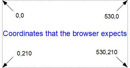
The top left hand of the screen is the origin or 0,0 point and as we go left or down the corresponding x and y values increase to the full values defined by height and width.
That’s good enough for the time values on the x axis that will start at lower values and increase, but for the values on the y axis we’re trying to go against the flow. We want the low values to be at the bottom and the high values to be at the top.
No problem. We just tell D3 via the statement y = d3.scale.linear().range([height, 0]); that the larger values (height) are at the low end of the screen (at the top) and the low values are at the bottom (as you most probably will have guessed by this stage, the .range statement uses the format .range([closer_to_the_origin, further_from_the_origin]). So when we put the height variable first, that is now associated at the top of the screen.
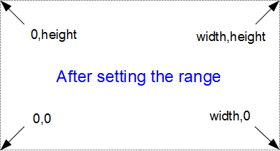
We’ve scaled our data to the graph size and ensured that the range of values is set appropriately. What’s with the domain part that was in this section’s title?
Come on, you remember this little piece of script don’t you?
x.domain(d3.extent(data, function(d) { return d.dtg; }));
y.domain([0, d3.max(data, function(d) { return d.temperature; })]);
While it exists in a separate part of the file from the scale / range part, it is certainly linked.
That’s because there’s something missing from what we have been describing so far with the set up of the data ranges for the graphs. We haven’t actually told D3 what the range of the data is.
So, the .domain function is designed to let D3 know what the scope of the data will be. This is what is then passed to the scale function.
Looking at the first part that is setting up the x axis values, it is saying that the domain for the x axis values will be determined by the d3.extent function which in turn is acting on a separate function which looks through all the ‘date’ values that occur in the ‘data’ array. In this case the .extent function returns the minimum and maximum value in the given array.
-
function(d) { return d.dtg; }returns all the ‘dtg’ values in ‘data’. This is then passed to… - The
.extentfunction that finds the maximum and minimum values in the array and then… - The
.domainfunction which returns those maximum and minimum values to D3 as the range for the x axis.
Pretty neat really. At first you might think it was overly complex, but breaking the function down into these components allows additional functionality with differing scales, values and quantities. In short, don’t sweat it. It’s a good thing.
Setting up the Axes
Now we come to our next piece of code;
var xAxis = d3.svg.axis().scale(x)
    .orient("bottom");

var yAxis = d3.svg.axis().scale(y)
    .orient("left").ticks(5);
I’ve included both the x and y axes because they carry out the formatting in very similar ways. It’s worth noting that this is not the point where the axes get drawn. That occurs later in the script.
D3 has it’s own axis component that aims to take the fuss out of setting up and displaying the axes. So it includes a number of configurable options.
Looking first at the x axis;
var xAxis = d3.svg.axis().scale(x)
    .orient("bottom");
The axis function is called with d3.svg.axis(). Then the scale is set using the x values that we set up in the scales, ranges and domains section using .scale(x). Then we tell the graph to orientate itself to the bottom of the graph .orient("bottom").
The code that formats the y axis is pretty similar;
var yAxis = d3.svg.axis().scale(y)
    .orient("left").ticks(5);
The only significant difference is that we define the number of ticks we would like to have on that axis (for the x axis we just let D3 pick an appropriate number)
Adding data to the line function
We’re getting towards the end of our journey through the script now. The next step is to get the information from the array ‘data’ and to place it in a new array that consists of a set of coordinates that we are going to plot.
var valueline = d3.svg.line()
    .x(function(d) { return x(d.dtg); })
    .y(function(d) { return y(d.temperature); });
I’m aware that the statement above may be somewhat ambiguous. You would be justified in thinking that we already had the data stored and ready to go. But that’s not strictly correct.
What we have is data in a raw format, we have added pieces of code that will allow the data to be adjusted for scale and range to fit in the area that we want to draw, but we haven’t actually taken our raw data and adjusted it for our desired coordinates. That’s what the code above does.
The main function that gets used here is the d3.svg.line() function. This function uses accessor functions to store the appropriate information in the right area and in the case above they use the x and y accessors (that would be the bits that are .x and .y). The d3.svg.line() function is called a ‘path generator’ and this is an indication that it can carry out some pretty clever things on its own accord. But in essence its job is to assign a set of coordinates in a form that can be used to draw a line.
Each time this line function is called on, it will go through the data and will assign coordinates to ‘dtg’ and ‘temperature’ pairs using the ‘x’ and ‘y’ functions that we set up earlier (which of course are responsible for scaling and setting the correct range / domain).
Of course, it doesn’t get the data all by itself, we still need to actually call the valueline function with ‘data’ as the source to act on. But never fear, that’s coming up soon.
Adding the SVG area.
As the title states, the next piece of script forms and adds the space that D3 will then use to draw on.
var svg = d3.select("body")
    .append("svg")
        .attr("width", width + margin.left + margin.right)
        .attr("height", height + margin.top + margin.bottom)
    .append("g")
        .attr("transform",
              "translate(" + margin.left + "," + margin.top + ")");
So what exactly does that all mean?
Well D3 needs to be able to have a space defined for it to draw things. When you define the space it’s going to use, you can also give it an identifying name and attributes.
In the example we’re using here, we are ‘appending’ an SVG element (an element that we are going to draw things on) to the <body> element of the HTML page.
We also add an element ‘g’ that is referenced to the top left corner of the actual graph area on the canvas. ‘g’ is actually a grouping element in the sense that it is normally used for grouping together several related elements. So in this case those grouped elements will have a common reference.
Interesting things to note about the code. The .attr(“stuff in here”) parts are attributes of the appended elements they are part of.
For instance;
    .append("svg")
        .attr("width", width + margin.left + margin.right)
        .attr("height", height + margin.top + margin.bottom)
tells us that the ‘svg’ element has a “width” of width + margin.left + margin.right and the “height” of height + margin.top + margin.bottom.
Likewise…
    .append("g")
        .attr("transform",
              "translate(" + margin.left + "," + margin.top + ")");
tells us that the element “g” has been transformed by moving(translating) to the point margin.left, margin.top. Or to the top left of the graph space proper. This way when we tell something to be drawn on our canvas, we can use the reference point “g” to make sure everything is in the right place.
Actually Drawing Something!
Up until now we have spent a lot of time defining, loading and setting up. Good news! We’re about to finally draw something!
We jump lightly over some of the code that we have already explained and land on the part that draws the line.
svg.append("path")
	.attr("d", valueline(data));
This area occurs in the part of the code that has the data loaded and ready for action.
The svg.append("path") portion adds a new path element . A path element represents a shape that can be manipulated in lots of different ways (see more here: http://www.w3.org/TR/SVG/paths.html). In this case it inherits the ‘path’ styles from the CSS section and on the following line (.attr("d", valueline(data));) we add the attribute “d”.
This is an attributer that stands for ‘path data’ and sure enough the valueline(data) portion of the script passes the ‘valueline’ array (with its x and y coordinates) to the path element. This then creates a svg element which is a path going from one set of ‘valueline’ coordinates to another.
Then we get to draw in the axes;
svg.append("g")
	.attr("class", "x axis")
	.attr("transform", "translate(0," + height + ")")
	.call(xAxis);

svg.append("g")
	.attr("class", "y axis")
	.call(yAxis);
We have covered the formatting of the axis components earlier. So this part is actually just about getting those components drawn onto our canvas.
Both axes start by being appended to the “g” group. Then each has its own classes applied for styling via CSS.
Feel free to mess about with these CSS styles to change the appearance of your axes.
On the x axis, we have a transform statement (.attr("transform", "translate(0," + height + ")")). If you recall, our point of origin for drawing is in the top left hand corner. Therefore if we want our x axis to be on the bottom of the graph, we need to move (transform) it to the bottom by a set amount. The set amount in this case is the height of the graph proper (height).
The last part of the two sections of script ( .call(xAxis); and .call(yAxis); ) call the x and y axis functions and initiate the drawing action.
Wrap Up
Well that’s it. In theory, you should now be a complete D3 ninja.
OK, perhaps a slight exaggeration. In fact there is a strong possibility that the information I have laid out here is at best borderline useful and at worst laden with evil practices and gross inaccuracies.
But look on the bright side. Irrespective of the nastiness of the way that any of it was accomplished or the inelegance of the code, if the picture drawn on the screen is relatively pretty, you can walk away with a smile. :-)
This section concludes a very basic description of one type of a graphic that can be built with D3. We will look at adding value to it in subsequent chapters.
Those with a smattering of knowledge of any of the topics I have butchered above (or below) are fully justified in feeling a large degree of righteous indignation. To those I say, please feel free to amend where practical and possible, but please bear in mind this was written from the point of view of someone with no experience in the topic and therefore try to keep any instructions at a level where a new entrant can step in.