Leanpub: Publish Early, Publish Often

Mapping with d3.js

Another string to the bow of d3.js is the addition of a set of powerful routines for handling geographical information.

In the same sense that a line graph is a simple representation of data on a document, a map can be regarded as a set of points with an underlying coordinate system. When you say it like that it seems obvious that it should be applied as a document for display. However, I don’t want to give the impression that this is some sort of trivial matter for either the original developers or for you, the person who wants to display a map. Behind the scenes for this type of work, the thought that must have gone into making the code usable and extensible must have been enormous.

Mike Bostock has lauded the work of Jason Davies in the development of the latest major version of d3.js (version 3) for his work on improving mapping capability. A visit to his home page provides a glimpse into Jason’s expertise and no visit would be complete without marvelling at his work with geographic projections.

Examples

I am firmly of the belief that mapping in particular has an enormous potential for adding value to data sets. The following collection of examples gives a brief taste of what has been accomplished by combining geographic information and D3 thus far. (The screen shots following have been sourced from the biovisualize gallery and as such provide attribution to the best of my ability. If I have incorrectly attributed the source or author please let me know and I will correct it promptly.)

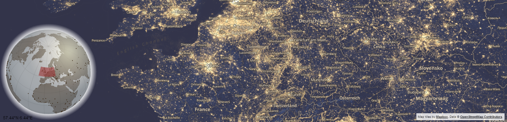
Faux D3 3d globe integrated with Mapbox / Open Street Map

Above is an interactive visualization showing the position of the main map on a faux D3 3d globe with a Mapbox / Open Street Map main window. Source dev.geosprocket.com Source Bill Morris.

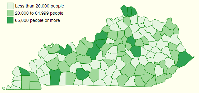
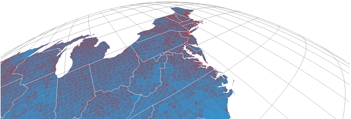
Kentucky Count Population from the 2010 census

This is a breakdown of population in Kentucky Counties from the 2010 census. Source: ccarpenterg.github.com by Cristian Carpenter.

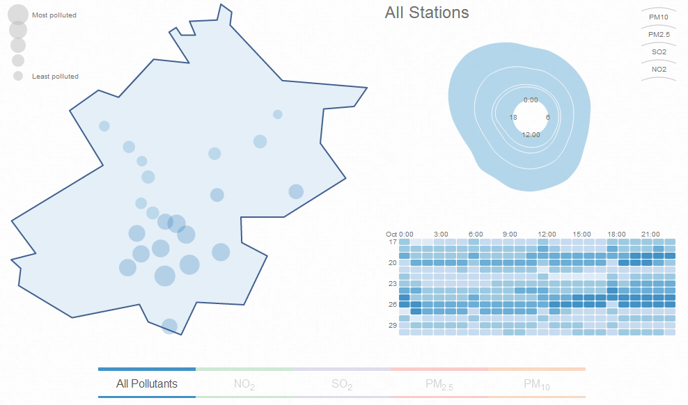
This map visualizes air pollution in Beijing. Source: scottcheng.github.com by Scott Cheng.

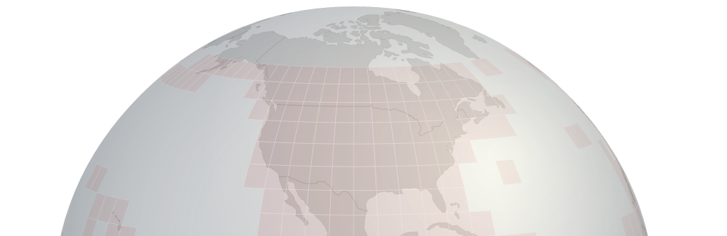
This is a section of the globe that is presented on the Shuttle Radar Topography Mission tile downloading web site. This excellent site uses the interactive globe to make the selection of SRTM tiles easy. Source dwtkns.com by Derek Watkins.

This is a static screen-shot of an animated tour of the Worlds countries. Source bl.ocks.org by Mike Bostock.

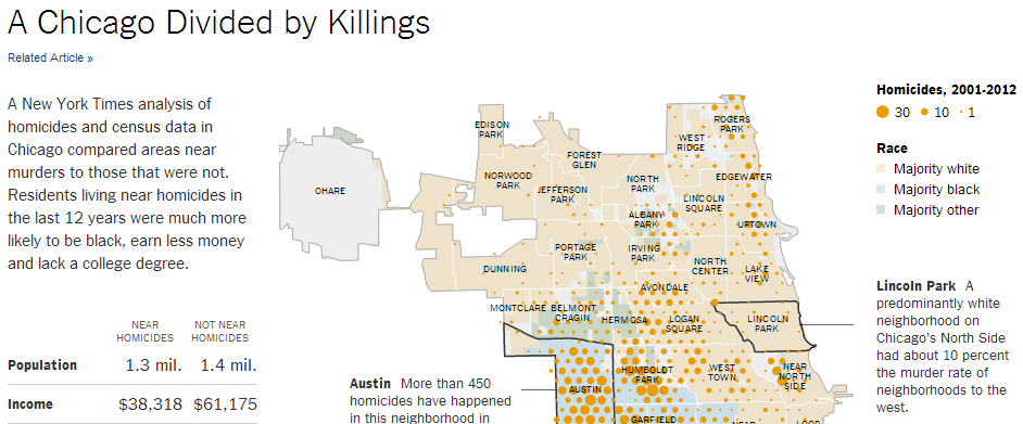
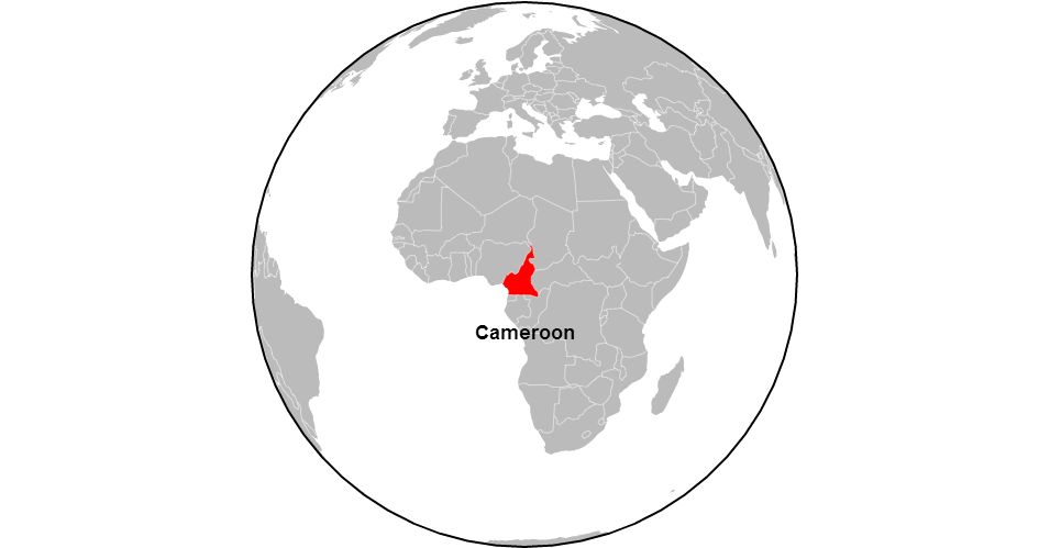
A Chicago Divided by Killings: New Your Times

This is one of the great infographics published by the New York Times. Source: www.nytimes.com by Mike Bostock, Shan Carter and Kevin Quealy.

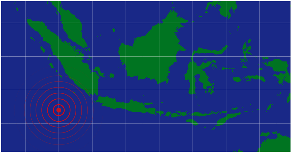
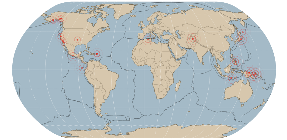
This is an animated graphic showing a series of concentric circles emanating from glowing red dot which was styled after a news article in The Onion. Source: bl.ocks.org by Mike Bostock.

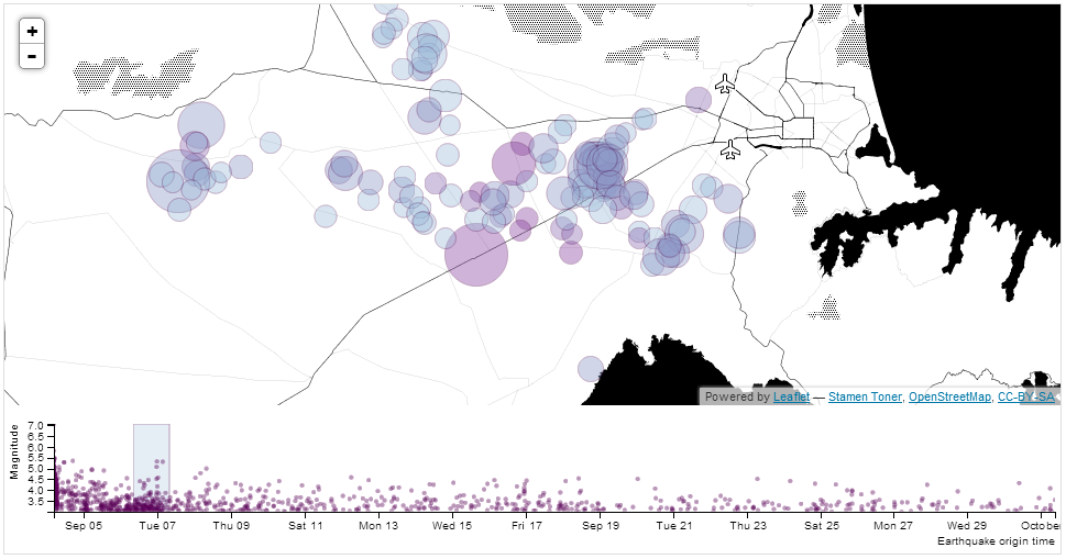
Here we see earthquakes represented on a selectable timeline where D3 generates a svg overlay and the map layer is created using Leaflet. Source: bl.ocks.org by tnightingale.

Carrying on with the earthquake theme, this is a map of all earthquakes in the past 24 hours over magnitude 2.5. Source: bl.ocks.org by benelsen.

An interactive satellite projection. Source dev.geosprocket.com by Bill Morris.

GeoJSON and TopoJSON

Projecting countries and various geographic features onto a map can be a very data hungry exercise. By that I mean that the information required to present geographic shapes can result in data files that are quite large. GeoJSON has been the default geographic data file of choice for quite some time, and as the name would suggest it encodes the data in a JSON type hierarchy. Often these GeoJSON files include a significant amount of extraneous detail or incorporate a level of accuracy that is impractical (too detailed).

Enter TopoJSON. Mike Bostock has designed TopoJSON as an extension to GeoJSON in the sense that it has a similar structure, but the geometries are not encoded discretely and where they share features, they are combined. Additionally TopoJSON encodes numeric values more efficiently and can incorporate a degree of simplification. This simplification can result in savings of file size of 80% or more depending on the area and use of compression. Although TopoJSON has only begun to be used, the advantages of it seem clear and so I will anticipate its future use by incorporating it in my example diagrams (not that the use of GeoJSON differs much if at all). A great description of TopoJSOn can be found on the TopoJSON wiki on github.

Starting with a simple map

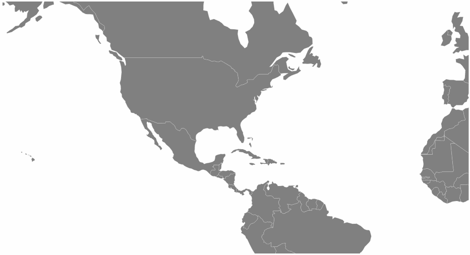
Our starting example will demonstrate the simple display of a World map. Our final result will looks like this;

The data file for the World map is one produced by Mike Bostock’s as part of his TopoJSON work.

We’ll move through the explanation of the code in a similar process to the one we went through when highlighting the function of the Sankey diagram. Where there are areas that we have covered before, I will gloss over some details on the understanding that you will have already seen them explained in an earlier section (most likely the basic line graph example).

The full code for this graphic can be found on github or in the code samples bundled with this book (world-map.html and world-110m2). A live example can be found on bl.ocks.org.

Here is the full code;

<!DOCTYPE html>
<meta charset="utf-8">
<style>

path {
  stroke: white;
  stroke-width: 0.25px;
  fill: grey;
}

</style>
<body>
<script src="http://d3js.org/d3.v3.min.js"></script>
<script src="http://d3js.org/topojson.v0.min.js"></script>
<script>

var width = 960,
    height = 500;

var projection = d3.geo.mercator()
    .center([0, 5 ])
    .scale(150)
    .rotate([-180,0]);

var svg = d3.select("body").append("svg")
    .attr("width", width)
    .attr("height", height);

var path = d3.geo.path()
    .projection(projection);

var g = svg.append("g");

// load and display the World
d3.json("world-110m2.json", function(error, topology) {
    g.selectAll("path")
      .data(topojson.object(topology, topology.objects.countries)
          .geometries)
    .enter()
      .append("path")
      .attr("d", path)
});

</script>
</body>
</html>

One of the first things that struck me when I first saw the code to draw a map was how small it was (the amount of code, not the World). It’s a measure of the degree of abstraction that D3 is able to provide to the process of getting data from a raw format to the screen that such a complicated task can be condensed to such an apparently small amount of code. Of course that doesn’t tell the whole story. Like a duck on a lake, above the water all is serene and calm while below the water the feet are paddling like fury. In this case, our code looks serene because D3 is doing all the hard work :-).

The first block of our code is the start of the file and sets up our HTML.

<!DOCTYPE html>
<meta charset="utf-8">
<style>

This leads into our style declarations.

path {
  stroke: white;
  stroke-width: 0.25px;
  fill: grey;
}

We only state the properties of the path components which will make up our countries. Obviously we will fill them with grey and have a thin (0.25px) line around each one.

The next block of code loads the JavaScript files.

</style>
<body>
<script src="http://d3js.org/d3.v3.min.js"></script>
<script src="http://d3js.org/topojson.v0.min.js"></script>
<script>

In this case it’s d3 and topojson. We load topojson.v0.min.js as a separate file because it’s still fairly new. In other words it hasn’t been incorporated into the main d3.js code base (that’s an assumption on my part since it might exist in isolation or perhaps end up as a plug-in). Whatever the case, for the time being, it exists as a separate file.

Then we get into the JavaScript. The first thing we do is define the size of our map.

var width = 960,
    height = 500;

Then we get into one of the simple, but cool parts of making any map. Setting up the view.

var projection = d3.geo.mercator()
    .center([0, 5 ])
    .scale(150)
    .rotate([-180,0]);

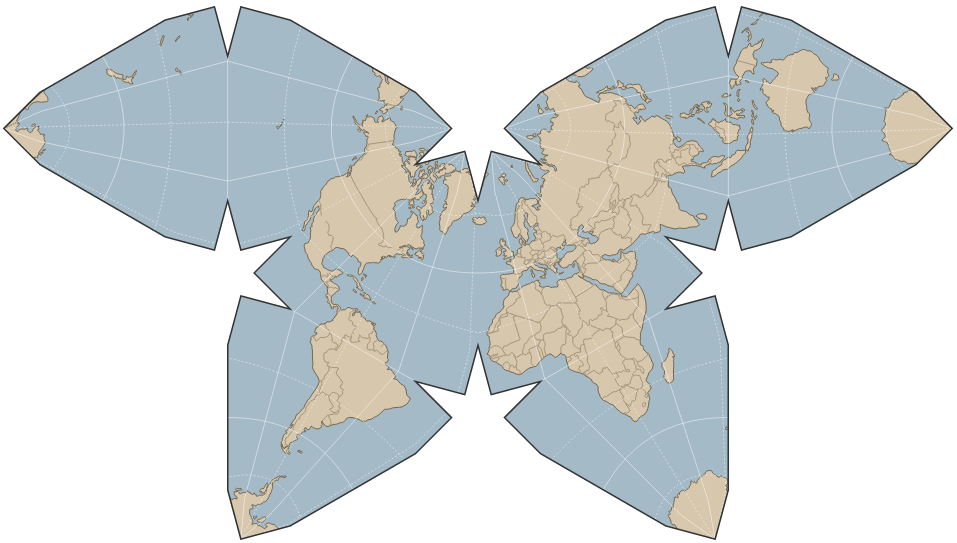
The projection is the way that the geographic coordinate system is adjusted for display on our flat screen. The screen is after all a two dimensional space and we are trying to present a three dimensional object. This is a big deal to cartographers in the sense that selecting a geographic projection for a map is an exercise in compromise. You can make it look pretty, but in doing so you can grievously distort the land size / shape. On the other hand you might make it more accurate, in size / shape but people will have trouble recognising it because they’re so used to the standard Mercator projection. For example, the awesome Waterman Butterfly.

There are a lot of alternatives available. Please have a browse on the wiki where you will find a huge range of options (66 at time of writing).

In our case we’ve gone with the conservative Mercator option.

Then we define three aspects of the projection. Center, scale and rotate.

center

If center is specified, this sets the projection’s center to the specified location as a two-element array of longitude and latitude in degrees and returns the projection. If center is not specified the default of (0°,0°) is used.

Our example is using [0, 5 ] which I have selected as being in the middle (I use 0) for longitude (left to right) and 5 degrees North of the equator (for latitude, North is positive, South is negative). This was purely to make it look aesthetically pleasing. Here’s the result of setting the center to [100,30].

The map has been centered on 100 degrees West and 30 degrees North. Of course, it’s also been pushed to the left without the right hand side of the map scrolling around. We’ll get to that in a moment.

scale

If scale is specified, this sets the projection’s scale factor to the specified value. If scale is not specified, it returns the current scale factor which defaults to 150. It’s important to note that scale factors are not consistent across projections.

Our current map uses a scale of 900. Again, this has been set for aesthetics. Keeping our center of [100,30], if we increase our scale to 2000 this is the result.

rotate

If rotation is specified, this sets the projection’s three-axis rotation to the specified angles for yaw, pitch and roll (equivalently longitude, latitude and roll) in degrees and returns the projection. If rotation is not specified, it sets the values to [0, 0, 0]. If the specified rotation has only two values, rather than three, the roll is assumed to be 0°.

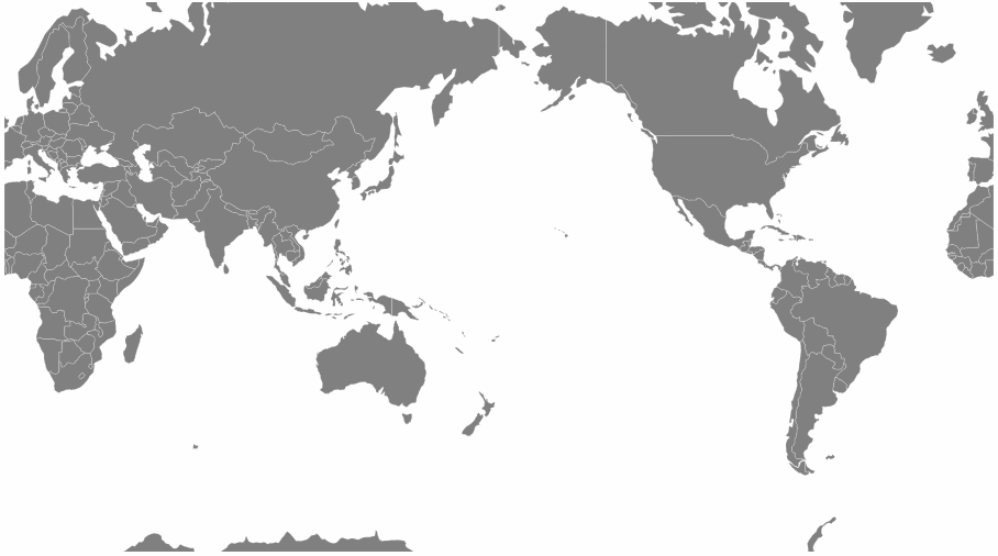
In our map we have specified [-180,0] so we can assume a roll value of zero. Likewise we have rotated our map by -180 degrees in longitude. This has been done specifically to place the map with the center on the anti-meridian (The international date line in the middle of the Pacific Ocean). If we return the value to [0,0](with our original values of scale and center this is the result.

In this case the centre of the map lines up with the meridian.

The next block of code sets our svg window;

var svg = d3.select("body").append("svg")
    .attr("width", width)
    .attr("height", height);

The following portion of code creates a new geographic path generator;

var path = d3.geo.path()
    .projection(projection);

The path generator (d3.geo.path()) is used to specify a projection type (.projection) which was defined earlier as a Mercator projection via the variable projection. (I’m not entirely sure, but it is possible that I have just set some kind of record for use of the word ‘projection’ in a sentence.)

We then declare g as our appended svg.

var g = svg.append("g");

The last block of JavaScript draws our map.

d3.json("world-110m2.json", function(error, topology) {
    g.selectAll("path")
      .data(topojson.object(topology, topology.objects.countries)
          .geometries)
    .enter()
      .append("path")
      .attr("d", path)
});

We load the TopoJSON file with the coordinates for our World map (world-110m2.json). Then we declare that we are going to act on all the path elements in the graphic (g.selectAll("path")).

Then we pull the data that defines the countries from the TopoJSON file (.data(topojson.object(topology, topology.objects.countries).geometries)). We add it to the data that we’re going to display (.enter()) and then we append that data as path elements (.append("path")).

The last html block closes off our tags and we have a map!

Zooming and panning a map

With our map displayed nicely we need to be able to move it about to explore it fully . To do this we can provide the functionality to zoom and pan it using the mouse.

Towards the end of the script, just before the close off of the script at the </script> tag we can add in the following code;

var zoom = d3.behavior.zoom()
    .on("zoom",function() {
        g.attr("transform","translate("+ 
            d3.event.translate.join(",")+")scale("+d3.event.scale+")");
        g.selectAll("path")  
            .attr("d", path.projection(projection)); 
});

svg.call(zoom)

This block of code introduces the behaviors functions. Using the d3.behavior.zoom function creates event listeners (which are like hidden functions standing by to look out for a specific type of activity on the computer and in this case mouse actions) to handle zooming and panning gestures on a container element (in this case our map). More information on the range of zoom options is available on the D3 Wiki.

We begin by declaring the zoom function as d3.behavior.zoom.

Then we instruct the computer that when it ‘sees’ a ‘zoom’ event to carry out another function (.on("zoom",function() {).

That function firstly gathers the (correctly formatted) translate and scale attributes in…

        g.attr("transform","translate("+ 
            d3.event.translate.join(",")+")scale("+d3.event.scale+")");

… and then applies them to all the path elements (which are the shapes of the countries) via…

        g.selectAll("path")  
            .attr("d", path.projection(projection));

Lastly we call the zoom function.

svg.call(zoom)

Then we relax and explore our map!

The full code for this graphic can be found on github or in the code samples bundled with this book (world-map-zoom-pan.html and world-110m2). A live example can be found on bl.ocks.org.

Displaying points on a map

Displaying maps and exploring them is pretty entertaining, but as anyone who has participated in the improvement of our geographic understanding of our world via projects such as Open Street Map will tell you, there’s a whole new level of cool to be attained by adding to a map.

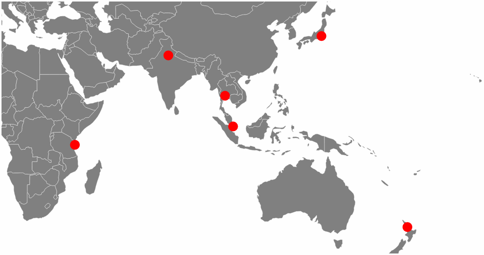
With that in mind, our next task is to add some simple detail in the form of points that show the location of cities.

To do this we will load in a csv file with data that identifies our cities and includes latitude and longitude details. Our file is called cities.csv and looks like this;

code,city,country,lat,lon
ZNZ,ZANZIBAR,TANZANIA,-6.13,39.31
TYO,TOKYO,JAPAN,35.68,139.76
AKL,AUCKLAND,NEW ZEALAND,-36.85,174.78
BKK,BANGKOK,THAILAND,13.75,100.48
DEL,DELHI,INDIA,29.01,77.38
SIN,SINGAPORE,SINGAPOR,1.36,103.75
BSB,BRASILIA,BRAZIL,-15.67,-47.43
RIO,RIO DE JANEIRO,BRAZIL,-22.90,-43.24
YTO,TORONTO,CANADA,43.64,-79.40
IPC,EASTER ISLAND,CHILE,-27.11,-109.36
SEA,SEATTLE,USA,47.61,-122.33

While we’re only going to use the latitude and longitude for our current work, the additional details could just as easily be used for labelling or tooltips.

We need to place our code carefully in this case because while you might have some flexibility in getting the right result with a locally hosted version of a map, there is a possibility that with a version hosted in the outside World (gasp the internet) you could strike trouble.

The code to load the cities should be placed inside the function that is loading the World map as indicated below;

d3.json("world-110m2.json", function(error, topology) {
    g.selectAll("path")
      .data(topojson.object(topology, topology.objects.countries)
          .geometries)
    .enter()
      .append("path")
      .attr("d", path)
                           // <== Put the new code block here
});

Here’s the new code;

    d3.csv("cities.csv", function(error, data) {
        g.selectAll("circle")
           .data(data)
           .enter()
           .append("circle")
           .attr("cx", function(d) {
                   return projection([d.lon, d.lat])[0];
           })
           .attr("cy", function(d) {
                   return projection([d.lon, d.lat])[1];
           })
           .attr("r", 5)
           .style("fill", "red");

We’ll go through the code and then explain the quirky thing about it.

First of all we load the cities.csv file (d3.csv("cities.csv", function(error, data) {). Then we select all the circle elements ( g.selectAll("circle")), assign our data (.data(data)), enter our data ( .enter()) and then add in circles (.append("circle")).

Then we set the x and y position for the circles based on the longitude (([d.lon, d.lat])[0]) and latitude (([d.lon, d.lat])[1]) information in the csv file.

Finally we assign a radius of 5 pixels and fill the circles with red.

The quirky thing about the new code block is that we have to put it inside the code block that loads the world data (d3.json("world-110m2.json", function(error, topology) {). We could place the two blocks one after the others (load / draw the world data, then load / draw the circles). And this will probably work if you run the file from your local computer. But when you host the files on the internet, it takes too long to load the world data compared to the city data and the end result is that the city data gets drawn before the world data and this is the result.

To avoid the problem we place the loading of the city data into the code that loads the World data. That way the city data doesn’t get loaded until the World data is loaded and then the circles get drawn on top of the world instead of under it :-).

The full code for this graphic can be found on github or in the code samples bundled with this book (world-map-cities.html, cities.csv and world-110m2). A live example can be found on bl.ocks.org.

Additionally the full code can be found in the appendix section at the rear of the book.

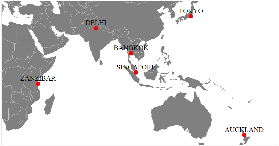
As an added extra and in response to a question that was asked on the d3noob.org blog, the names of the cities can be placed alongside the location dots by the addition of the following block of code inside the ‘cities’ loading portion of the script;

    g.selectAll("text")
       .data(data)
       .enter()
     .append("text") // append text
       .attr("x", function(d) {
               return projection([d.lon, d.lat])[0];
       })
       .attr("y", function(d) {
               return projection([d.lon, d.lat])[1];
       })
       .attr("dy", -7) // set y position of bottom of text
      .style("fill", "black") // fill the text with the colour black
      .attr("text-anchor", "middle") // set anchor y justification
      .text(function(d) {return d.city;}); // define the text to display

The end result shows the name of the cities placed above and centred with respect to the location.

The full code for this graphic can be found on github or in the code samples bundled with this book (world-map-cities-text.html, cities.csv and world-110m2). A live example can be found on bl.ocks.org.

Making maps with d3.js and leaflet.js combined

If you’ve read to this point in D3 Tips and Tricks, you may be aware that I have also written another book called ‘Leaflet Tips and Tricks’. I haven’t written both books because they are integrated with each other or because they seem made to compliment each other. I wrote them because both libraries are the best of breed (IMHO) at what they do. It should come as little surprise that they can have a lot to offer users who want to combine the incredible scope of d3.js’s data manipulation functions and the elegance of leaflet.js’s tile map presentation capabilities.

leaflet.js Overview

Leaflet.js is an Open Source JavaScript library designed to make deploying maps on a web page easy. It uses a paltry 34kB (at time of writing) JavaScript file that loads with your web page and provides access to a range of functions that will allow you to present a map.

Its goals are to be simple to use while focussing on performance and usability, but it’s also built to be extended using plugins that extend its functionality. It has an excellent API which is well documented, so there are no mysteries to using it successfully in a range of situations.

Out of the box Leaflet provides the functionality to add markers, popups, overlay lines and shapes, use multiple layers, zoom, pan and generally have a good time :-). But these are just the the core features of Leaflet. One of the significant strengths of Leaflet is the ability to extend the functionality of the script with plugins from third parties. At the time of writing there are over 80 separate plugins that allow features such as overlaying a heatmap, animating markers, loading csv files of data, drawing complex shapes, measuring distance, manipulating layers and displaying coordinates.

Leaflet is simple, elegant and functional but powerful. There’s a good chance that even if you don’t present maps with Leaflet, you’ll be using ones that someone else made with it at some stage on the Internet.

Why use leaflet.js when d3.js does maps too?

Good question. I can see you’ve been paying attention.

There is a significant difference between the underlying way that d3.js and leaflet.js presents mapping data. D3.js predominantly focusses on vector based graphics when drawing maps and leaflet.js leverages the huge range of bitmap based map tiles that are available for use around the world. Both bitmap and vector based solutions have strengths and weaknesses depending on the application. Combining both allows the use of the best of both worlds.

Leaflet map with d3.js objects that scale with the map

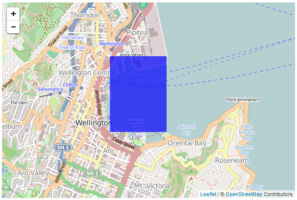
The first example we’ll look at will project a leaflet.js map on the screen with a d3.js object (in this case a simple rectangle) onto the map.

The rectangle will be bound to a set of geographic coordinates so that as the map is panned and zoomed the rectangle will shrink and grow. For example the following diagram shows a rectangle (made with d3.js ) superimposed over a leaflet.js map;

If we then zoom in…

Zoomed rectangular d3 area on leaflet map

…the rectangle zooms in as well.

This may not sound terribly exciting and if you’re familiar with Leaflet you will know that it is possible to draw polygons onto a map using only leaflet’s built in functions. However, the real strength of this application of vector data comes when making the d3.js content interactive which is more difficult with leaflet.js.

For an excellent example of this please visit Mike Bostock’s tutorial where he demonstrates superimposing a map of the United States separated by state (which react individually to the mouse being hovered over them). My following explanation is a humble derivation of his code.

Speaking of code, here is a full listing of the code that we will be using;

<!DOCTYPE html>
<html>
<head>
    <title>Leaflet and D3 Map</title>
    <meta charset="utf-8" />
    <link 
        rel="stylesheet" 
        href="http://cdn.leafletjs.com/leaflet-0.7/leaflet.css"
    />
    
</head>
<body>

    <div id="map" style="width: 600px; height: 400px"></div>

	<script src="http://d3js.org/d3.v3.min.js"></script>

    <script
        src="http://cdn.leafletjs.com/leaflet-0.7/leaflet.js">
    </script>

    <script>
	
        var map = L.map('map').setView([-41.2858, 174.7868], 13);
        mapLink = 
            '<a href="http://openstreetmap.org">OpenStreetMap</a>';
        L.tileLayer(
            'http://{s}.tile.openstreetmap.org/{z}/{x}/{y}.png', {
            attribution: '&copy; ' + mapLink + ' Contributors',
            maxZoom: 18,
            }).addTo(map);

		// Add an SVG element to Leaflet’s overlay pane
		var svg = d3.select(map.getPanes().overlayPane).append("svg"),
			g = svg.append("g").attr("class", "leaflet-zoom-hide");
			
		d3.json("rectangle.json", function(geoShape) {
		
		//  create a d3.geo.path to convert GeoJSON to SVG
		var transform = d3.geo.transform({point: projectPoint}),
            path = d3.geo.path().projection(transform);
 
		// create path elements for each of the features
		d3_features = g.selectAll("path")
			.data(geoShape.features)
			.enter().append("path");

		map.on("viewreset", reset);

		reset();

		// fit the SVG element to leaflet's map layer
		function reset() {
        
			bounds = path.bounds(geoShape);

			var topLeft = bounds[0],
				bottomRight = bounds[1];

			svg .attr("width", bottomRight[0] - topLeft[0])
				.attr("height", bottomRight[1] - topLeft[1])
				.style("left", topLeft[0] + "px")
				.style("top", topLeft[1] + "px");

			g .attr("transform", "translate(" + -topLeft[0] + "," 
			                                  + -topLeft[1] + ")");

			// initialize the path data	
			d3_features.attr("d", path)
				.style("fill-opacity", 0.7)
				.attr('fill','blue');
		} 

		// Use Leaflet to implement a D3 geometric transformation.
		function projectPoint(x, y) {
			var point = map.latLngToLayerPoint(new L.LatLng(y, x));
			this.stream.point(point.x, point.y);
		}

	})
        
    </script>
</body>
</html>

There is also an associated json data file (called rectangle.json) that has the following contents;

{
"type": "FeatureCollection",
"features": [ { 
	"type": "Feature", 
	"geometry": { 
		"type": "Polygon", 
		"coordinates": [ [ 
		[ 174.78, -41.29 ], 
		[ 174.79, -41.29 ], 
		[ 174.79, -41.28 ], 
		[ 174.78, -41.28 ], 
		[ 174.78, -41.29 ] 
		] ] 
		}
	}	
]
}

The full code and a live example are available online at bl.ocks.org or GitHub. They are also available as the files ‘leaflet-d3-combined.html’ and ‘rectangle.json’ as a separate download with D3 Tips and Tricks. A a copy of all the files that appear in the book can be downloaded (in a zip file) when you download the book from Leanpub

While I will explain the code below, please be aware that I will gloss over some of the simpler sections that are covered in other sections of either books and will instead focus on the portions that are important to understand the combination of d3 and leaflet.

Our code begins by setting up the html document in a fairly standard way.

<!DOCTYPE html>
<html>
<head>
    <title>Leaflet and D3 Map</title>
    <meta charset="utf-8" />
    <link 
        rel="stylesheet" 
        href="http://cdn.leafletjs.com/leaflet-0.7/leaflet.css"
    />
    
</head>
<body>

    <div id="map" style="width: 600px; height: 400px"></div>

	<script src="http://d3js.org/d3.v3.min.js"></script>

    <script
        src="http://cdn.leafletjs.com/leaflet-0.7/leaflet.js">
    </script>

Here we’re getting some css styling and loading our leaflet.js / d3.js libraries. The only configuration item is where we set up the size of the map (in the <style> section and as part of the map div).

Then we break into the JavaScript code. The first thing we do is to project our Leaflet map;

var map = L.map('map').setView([-41.2858, 174.7868], 13);
mapLink = 
	'<a href="http://openstreetmap.org">OpenStreetMap</a>';
L.tileLayer(
	'http://{s}.tile.openstreetmap.org/{z}/{x}/{y}.png', {
	attribution: '&copy; ' + mapLink + ' Contributors',
	maxZoom: 18,
	}).addTo(map);

This is exactly the same as we have done in any of the simple map explanations in Leaflet Tips and Tricks and in this case we are using the OpenStreetMap tiles.

Then we start on the d3.js part of the code.

The first part of that involves making sure that Leaflet and D3 are synchronised in the view that they’re projecting. This synchronisation needs to occur in zooming and panning so we add an SVG element to Leaflet’s overlayPlane

var svg = d3.select(map.getPanes().overlayPane).append("svg"),
	g = svg.append("g").attr("class", "leaflet-zoom-hide");

Then we add a g element that ensures that the SVG element and the Leaflet layer have the same common point of reference. Otherwise when they zoomed and panned it could be offset. The leaflet-zoom-hide affects the presentation of the map when zooming. Without it the underlying map zooms to a new size, but the d3.js elements remain as they are until the zoom effect has taken place and then they adjust. It still works fine, but it ‘looks’ wrong.

Then we load our data file with the line…

d3.json("rectangle.json", function(geoShape) {

This is pretty standard fare for d3.js but it’s worth being mindful that while the type of data file is .json this is a GeoJSON file and they have particular features (literally) that allow them to do their magic. There is a good explanation of how they are structured at geojson.org for those who are unfamiliar with the differences.

Using our data we need to ensure that it is correctly transformed from our latitude/longitude coordinates as supplied to coordinates on the screen. We do this by implementing d3’s geographic transformation features (d3.geo).

var transform = d3.geo.transform({point: projectPoint}),
	path = d3.geo.path().projection(transform);

Here the path that we want to create in SVG is generated from the points that are supplied from the data file which are converted by the function projectPoint This function (which is placed at the end of the file) takes our latitude and longitudes and transforms them to screen (layer) coordinates.

function projectPoint(x, y) {
	var point = map.latLngToLayerPoint(new L.LatLng(y, x));
	this.stream.point(point.x, point.y);
}

With the transformations now all taken care of we can generate our path in the traditional d3.js way and append it to our g group.

d3_features = g.selectAll("path")
	.data(geoShape.features)
	.enter().append("path");

The last ‘main’ part of our JavaScript makes sure that when our view of what we’re looking at changes (we zoom or pan) that our d3 elements change as well;

	map.on("viewreset", reset);

	reset();

Obviously when our view changes we call the function reset. It’s the job of the reset function to ensure that whatever the leaflet layer does, the SVG (d3.js) layer follows;

function reset() {

    bounds = path.bounds(geoShape);

    var topLeft = bounds[0],
        bottomRight = bounds[1];

    svg .attr("width", bottomRight[0] - topLeft[0])
        .attr("height", bottomRight[1] - topLeft[1])
        .style("left", topLeft[0] + "px")
        .style("top", topLeft[1] + "px");

    g .attr("transform", "translate(" + -topLeft[0] + "," 
                                      + -topLeft[1] + ")");

    // initialize the path data	
    d3_features.attr("d", path)
        .style("fill-opacity", 0.7)
        .attr('fill','blue');
}

It does this by establishing the topLeft and bottomRightcorners of the desired area and then it applies the width, height, top and bottom attributes to the svg element and translates the g element to the right spot. Last, but not least it redraws the path.

The end result being a fine combination of leaflet.js map and ds.js element;

Leaflet map with d3.js elements that are overlaid on a map

The next example of a combination of d3.js and leaflet.js is one where we want to have an element overlaid on our map at a specific location, but have it remain a specific size over the map. For example, here we will display 5 circles which are centred at specific geographic locations.

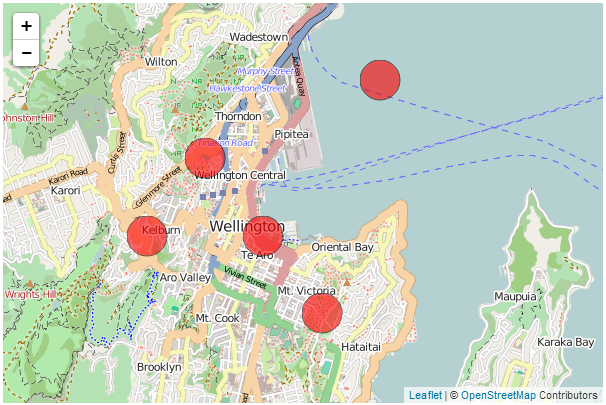
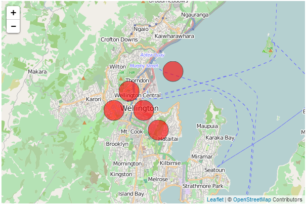
d3.js circles fixed in geographic location on leaflet map but constant size

When we zoom out of the map, those circles remain over the geographic location, but the same size on the screen.

Zoomed d3.js circles fixed in geographic location on leaflet map but constant size

You may (justifiably) ask yourself why we would want to do this with d3.js when Leaflet could do the same job with a marker? The answer is that as cool as leaflet.js’s markers are, d3 elements have a wider range of features that make their use advantageous in some situations. For instance if you want to animate or rotate the icons or dynamically adjust some of their attributes, d3.js would have a greater scope for adjustments.

The following code draws circles at geographic locations;

<!DOCTYPE html>
<html>
<head>
    <title>d3.js with leaflet.js</title>

    <link 
        rel="stylesheet" 
        href="http://cdn.leafletjs.com/leaflet-0.7/leaflet.css"
    />
    <script src="http://d3js.org/d3.v3.min.js"></script>

    <script
        src="http://cdn.leafletjs.com/leaflet-0.7/leaflet.js">
    </script>
    
</head>
<body>

    <div id="map" style="width: 600px; height: 400px"></div>

    <script type="text/javascript">
	
        var map = L.map('map').setView([-41.2858, 174.7868], 13);
        mapLink = 
            '<a href="http://openstreetmap.org">OpenStreetMap</a>';
        L.tileLayer(
            'http://{s}.tile.openstreetmap.org/{z}/{x}/{y}.png', {
            attribution: '&copy; ' + mapLink + ' Contributors',
            maxZoom: 18,
            }).addTo(map);
 
    // Initialize the SVG layer
    map._initPathRoot()    

    // We pick up the SVG from the map object
    var svg = d3.select("#map").select("svg"),
    g = svg.append("g");
	
    d3.json("circles.json", function(collection) {
        // Add a LatLng object to each item in the dataset
        collection.objects.forEach(function(d) {
            d.LatLng = new L.LatLng(d.circle.coordinates[0],
                                    d.circle.coordinates[1])
        })
		
        var feature = g.selectAll("circle")
            .data(collection.objects)
            .enter().append("circle")
            .style("stroke", "black")  
            .style("opacity", .6) 
            .style("fill", "red")
            .attr("r", 20);  
		
        map.on("viewreset", update);
        update();

        function update() {
            feature.attr("transform", 
            function(d) { 
                return "translate("+ 
                    map.latLngToLayerPoint(d.LatLng).x +","+ 
                    map.latLngToLayerPoint(d.LatLng).y +")";
                }
            )
        }
    })			 
</script>
</body>
</html>

There is also an associated json data file (called circles.json) that has the following contents;

{"objects":[
{"circle":{"coordinates":[-41.28,174.77]}},
{"circle":{"coordinates":[-41.29,174.76]}},
{"circle":{"coordinates":[-41.30,174.79]}},
{"circle":{"coordinates":[-41.27,174.80]}},
{"circle":{"coordinates":[-41.29,174.78]}}
]}

The full code and a live example are available online at bl.ocks.org or GitHub. They are also available as the files ‘leaflet-d3-linked.html’ and ‘circles.json’ as a separate download with D3 Tips and Tricks. A a copy of all the files that appear in the book can be downloaded (in a zip file) when you download the book from Leanpub

While I will explain the code below, as with the previous example (which is similar, but different) please be aware that I will gloss over some of the simpler sections that are covered in other sections of either books and will instead focus on the portions that are important to understand the combination of d3 and leaflet.

Our code begins by setting up the html document in a fairly standard way.

<!DOCTYPE html>
<html>
<head>
	<title>d3.js with leaflet.js</title>

    <link 
        rel="stylesheet" 
        href="http://cdn.leafletjs.com/leaflet-0.7/leaflet.css"
    />
    <script src="http://d3js.org/d3.v3.min.js"></script>

    <script
        src="http://cdn.leafletjs.com/leaflet-0.7/leaflet.js">
    </script>
    
</head>
<body>

	<div id="map" style="width: 600px; height: 400px"></div>

Here we’re getting some css styling and loading our leaflet.js / d3.js libraries. The only configuration item is where we set up the size of the map (in the <div> section and as part of the map div).

Then we break into the JavaScript code. The first thing we do is to project our Leaflet map;

    var map = L.map('map').setView([-41.2858, 174.7868], 13);
    mapLink = 
        '<a href="http://openstreetmap.org">OpenStreetMap</a>';
    L.tileLayer(
        'http://{s}.tile.openstreetmap.org/{z}/{x}/{y}.png', {
        attribution: '&copy; ' + mapLink + ' Contributors',
        maxZoom: 18,
        }).addTo(map);

This is exactly the same as we have done in any of the simple map explanations in Leaflet Tips and Tricks and in this case we are using the OpenStreetMap tiles.

Then we start on the d3.js part of the code.

Firstly the Leaflet map is initiated as SVG using map._initPathRoot().

	// Initialize the SVG layer
	map._initPathRoot()    

	// We pick up the SVG from the map object
	var svg = d3.select("#map").select("svg"),
	g = svg.append("g");

Then we select the svg layer and append a g element to give a common reference point g = svg.append("g").

Then we load the json file with the coordinates for the circles;

	d3.json("circles.json", function(collection) {

Then for each of the coordinates in the objects section of the json data we declare a new latitude / longitude pair from the associated coordinates;

	collection.objects.forEach(function(d) {
        d.LatLng = new L.LatLng(d.circle.coordinates[0],
                                d.circle.coordinates[1])
	})

Then we use a simple d3.js routine to add and place our circles based on the coordinates of each of our objects.

		var feature = g.selectAll("circle")
			.data(collection.objects)
			.enter().append("circle")
			.style("stroke", "black")  
			.style("opacity", .6) 
			.style("fill", "red")
			.attr("r", 20);

We declare each as a feature and add a bit of styling just to make them stand out.

The last ‘main’ part of our JavaScript makes sure that when our view of what we’re looking at changes (we zoom or pan) that our d3 elements change as well;

		map.on("viewreset", update);
		update();

Obviously when our view changes we call the function update. It’s the job of the update function to ensure that whenever the leaflet layer moves, the SVG layer with the d3.js elements follows and the points that designate the locations of those objects move appropriately;

	function update() {
		feature.attr("transform", 
		function(d) { 
			return "translate("+ 
				map.latLngToLayerPoint(d.LatLng).x +","+ 
				map.latLngToLayerPoint(d.LatLng).y +")";
			}
		)
	}

Here we are using the transform function on each feature to adjust the coordinates on our LatLng coordinates. We only need to adjust our coordinates since the size, shape, rotation and any other attribute or style is dictated by the objects themselves.

And there we have it!

Up next

D3.js Examples Explained