Force Layout Diagrams

What is a Force Layout Diagram?

This is not a distinct type of diagram per se. Instead, it’s a way of representing data so that individual data points share relationships to other data points via forces. Those forces can then act in different ways to provide a natural structure to the data. The end result can be a wide variety of representations of connectedness and groupings.

Mike Bostock gave a great talk which focussed on force layout techniques in 2011 at Trulia for the Data Visualization meetup group. Check video of the presentation here: http://vimeo.com/29458354 and the slides here: http://mbostock.github.com/d3/talk/20110921/#0. The most memorable quote I recall from the talk describes force layout diagrams as an “Implicit way to do position encoding”.

Here’s some examples for those who need a reason to view the talk.

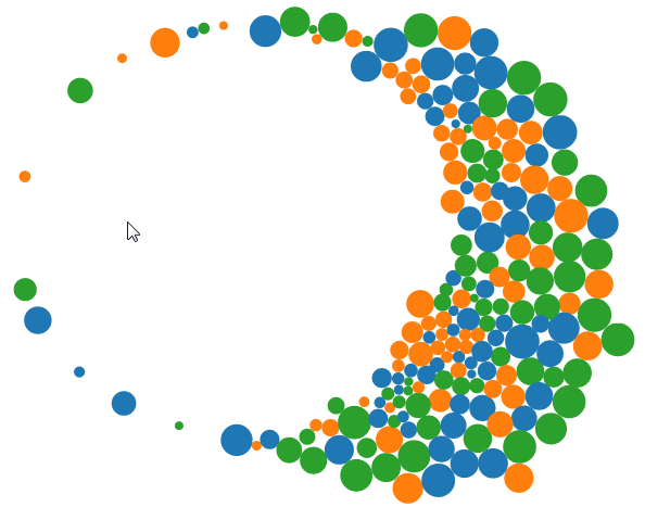
Multi-Foci Force Layout

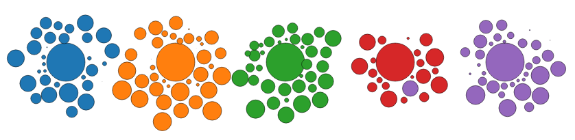
Simultaneous forces of repulsion and multiple gravitational focus points create a natural clustering of data points (Source: Mike Bostock http://bl.ocks.org/mbostock/1249681). The graph is animated, so the artefacts such as overlapping circles and the purple circle that is located beside the red area are transitory.

Force Directed Graph with Pan / Zoom

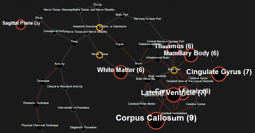
Multiple linked nodes show connections between related entities where those entities are labelled and encoded with relevant information. Created by David Graus and presented here: http://graus.nu/blog/force-directed-graphs-playing-around-with-d3-js/.

Collapsible Force Layout

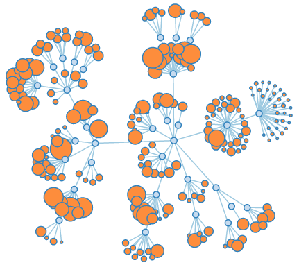
This force directed graph can have individual nodes expanded or collapsed by clicking on them to reveal or hide greater detail (Source: Mike Bostock http://bl.ocks.org/mbostock/1062288).

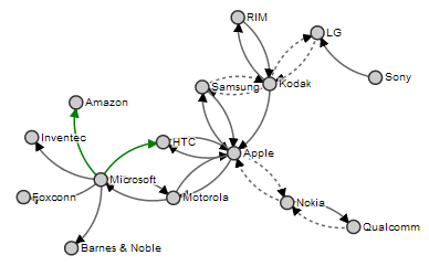
Force Directed Graph showing Directionality

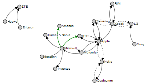
This example showing mobile patent lawsuits between companies presents the direction associated with the links and encodes the links to show different types (Source: Mike Bostock http://bl.ocks.org/mbostock/1153292).

Collision Detection

In this example the mouse exerts a repulsive force on the objects as it moves on the screen (Source: Mike Bostock http://bl.ocks.org/mbostock/3231298).

Molecule Diagram

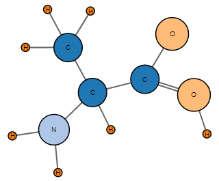
Just for fun, here is a diagram that Mike Bostock made to demonstrate drawing two parallel lines between nodes. He’s the first to admit that increasing the number of lines becomes awkward, but it serves as another example of the flexibility of force diagrams in D3 (Source: Mike Bostock http://bl.ocks.org/mbostock/3037015).

The main forces in play in these diagrams are charge, gravity and friction. More detailed information on these forces and the other parameters associated with the force layout code can be found in the D3 Wiki.

Charge

Charge is a force that a node can exhibit where it can either attract (positive values) or repel (negative values). Varying this value in conjunction with other forces (such as gravity) or a link (on a node by node basis) is generally necessary to maintain stability.

Gravity

The gravity force isn’t actually a true representation of gravitational attraction (this can be more closely approximated using positive values of charge). Instead it approximates the action of a spring connected to a node. This has a more pleasant visual effect when the affected node is closer to its ‘great attractor’ and avoids what would otherwise be a small black hole type effect.

Friction

The frictional force is one designed to act on the movement of a node to reduce its speed over time. It isn’t implemented as true friction (in the physical sense) and should be thought of as a ‘velocity decay’ in the truer sense.

Mike makes the point in the 2011 talk at Trulia that when using gravity in a force layout diagram, it is useful to include a degree of charge repulsion to provide stability. This can be demonstrated by experimenting with varying values of the charges in a diagram and observing the effects.

Force directed graph examples.

There are a large number of possible examples to use to demonstrate force directed graphs. I chose to combine two examples that Mike Bostock has demonstrated in the past. Both use the data for the ‘who’s suing who’ graph because I wanted especially to include the directionality aspect of the links. The two graphs I based the final graph on were the Mobile Patent Suits graph….

… for the directionality and link encoding and the Force-Directed Graph with Mouseover graph…

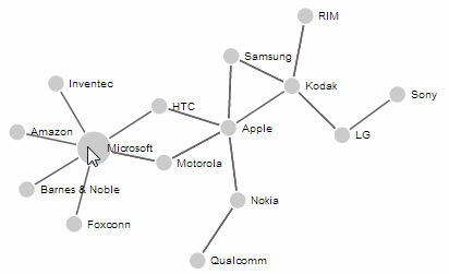
… for the mouseover effects (note the enlarged ‘Microsoft’ circle).

In spite of the similarities to each other in terms of data and network linkages, the final example code was quite different, so the end result is a distinct hybrid of the two and will look something like this;

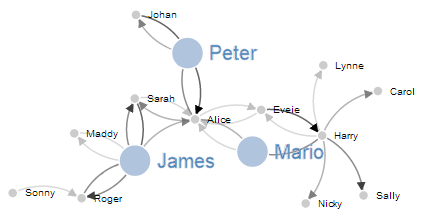
In this example the nodes can be clicked on once to enlarge the associated circle and text and then double clicked on to return them to normal. The links vary in opacity depending on an associated value loaded with the data. The example code for the graph above will be explained later in the chapter and can be found on bl.ocks.org or in the code samples bundled with this book (force-highlight-opacity.html and force.csv).

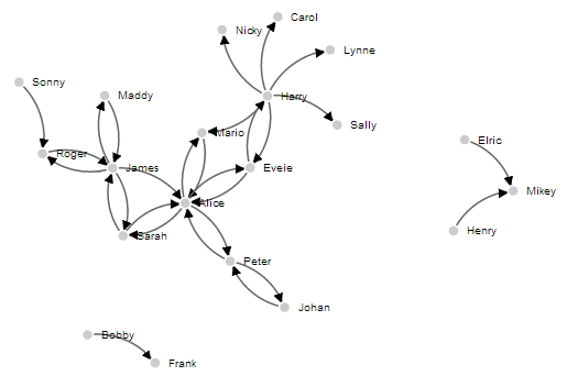
Basic force directed graph showing directionality

The data for this graph has been altered from the data that was comprised of litigants in the mobile patent war to fictitious people’s names and associated values (to represent the strength of the links between the two).

The full code for this diagram can also be found on github or in the code samples bundled with this book (force.html and force.csv). A live example can be found on bl.ocks.org.

In the original examples the data was contained in the graph code. In the following example it is loaded from a csv file. The values loaded are as follows;

source,target,value
Harry,Sally,1.2
Harry,Mario,1.3
Sarah,Alice,0.2
Eveie,Alice,0.5
Peter,Alice,1.6
Mario,Alice,0.4
James,Alice,0.6
Harry,Carol,0.7
Harry,Nicky,0.8
Bobby,Frank,0.8
Alice,Mario,0.7
Harry,Lynne,0.5
Sarah,James,1.9
Roger,James,1.1
Maddy,James,0.3
Sonny,Roger,0.5
James,Roger,1.5
Alice,Peter,1.1
Johan,Peter,1.6
Alice,Eveie,0.5
Harry,Eveie,0.1
Eveie,Harry,2.0
Henry,Mikey,0.4
Elric,Mikey,0.6
James,Sarah,1.5
Alice,Sarah,0.6
James,Maddy,0.5
Peter,Johan,0.7

The code is as follows;

<!DOCTYPE html>
<meta charset="utf-8">
<script src="http://d3js.org/d3.v3.js"></script>

<style>

path.link {
  fill: none;
  stroke: #666;
  stroke-width: 1.5px;
}

circle {
  fill: #ccc;
  stroke: #fff;
  stroke-width: 1.5px;
}

text {
  fill: #000;
  font: 10px sans-serif;
  pointer-events: none;
}

</style>
<body>
<script>

// get the data
d3.csv("force.csv", function(error, links) {

var nodes = {};

// Compute the distinct nodes from the links.
links.forEach(function(link) {
    link.source = nodes[link.source] || 
        (nodes[link.source] = {name: link.source});
    link.target = nodes[link.target] || 
        (nodes[link.target] = {name: link.target});
    link.value = +link.value;
});

var width = 960,
    height = 500;

var force = d3.layout.force()
    .nodes(d3.values(nodes))
    .links(links)
    .size([width, height])
    .linkDistance(60)
    .charge(-300)
    .on("tick", tick)
    .start();

var svg = d3.select("body").append("svg")
    .attr("width", width)
    .attr("height", height);

// build the arrow.
svg.append("svg:defs").selectAll("marker")
    .data(["end"])      // Different link/path types can be defined here
  .enter().append("svg:marker")    // This section adds in the arrows
    .attr("id", String)
    .attr("viewBox", "0 -5 10 10")
    .attr("refX", 15)
    .attr("refY", -1.5)
    .attr("markerWidth", 6)
    .attr("markerHeight", 6)
    .attr("orient", "auto")
  .append("svg:path")
    .attr("d", "M0,-5L10,0L0,5");

// add the links and the arrows
var path = svg.append("svg:g").selectAll("path")
    .data(force.links())
  .enter().append("svg:path")
    .attr("class", "link")
    .attr("marker-end", "url(#end)");

// define the nodes
var node = svg.selectAll(".node")
    .data(force.nodes())
  .enter().append("g")
    .attr("class", "node")
    .call(force.drag);

// add the nodes
node.append("circle")
    .attr("r", 5);

// add the text 
node.append("text")
    .attr("x", 12)
    .attr("dy", ".35em")
    .text(function(d) { return d.name; });

// add the curvy lines
function tick() {
    path.attr("d", function(d) {
        var dx = d.target.x – d.source.x,
            dy = d.target.y – d.source.y,
            dr = Math.sqrt(dx * dx + dy * dy);
        return "M" + 
            d.source.x + "," + 
            d.source.y + "A" + 
            dr + "," + dr + " 0 0,1 " + 
            d.target.x + "," + 
            d.target.y;
    });

    node
        .attr("transform", function(d) { 
		    return "translate(" + d.x + "," + d.y + ")"; });
}

});

</script>
</body>
</html>

In a similar process to the one we went through when highlighting the function of the Sankey diagram, where there are areas that we have covered before, I will gloss over some details on the understanding that you will have already seen them explained in an earlier section (most likely the basic line graph example).

The first block we come across is the initial html section;

<!DOCTYPE html>
<meta charset="utf-8">
<script src="http://d3js.org/d3.v3.js"></script>

<style>

The only thing slightly different with this example is that we load the d3.v3.js script earlier. This has no effect on running the code.

The next section loads the Cascading Style Sheets;

path.link {
  fill: none;
  stroke: #666;
  stroke-width: 1.5px;
}

circle {
  fill: #ccc;
  stroke: #fff;
  stroke-width: 1.5px;
}

text {
  fill: #000;
  font: 10px sans-serif;
  pointer-events: none;
}

We set styles for three elements and all the settings laid out are familiar to us from previous work.

Then we move into the JavaScript. Our first line loads our csv data file (force.csv).

d3.csv("force.csv", function(error, links) {

Then we declare an empty object (I still tend to think of these as arrays even though they’re strictly not).

var nodes = {};

This will contain our data for our nodes. We don’t have any separate node information in our data file, it’s just link information, so we will be populating this in the next section…

links.forEach(function(link) {
    link.source = nodes[link.source] || 
        (nodes[link.source] = {name: link.source});
    link.target = nodes[link.target] || 
        (nodes[link.target] = {name: link.target});
    link.value = +link.value;
});

This block of code looks through all of our data from our csv file and for each link adds it as a node if it hasn’t seen it before. It’s quite clever how it works as it employs a neat JavaScript shorthand method using the double pipe (||) identifier.

So the line (expanded)…

link.source=nodes[link.source] || (nodes[link.source]={name: link.source});

… can be thought of as saying “If link.source does not equal any of the nodes values then create a new element in the nodes object with the name of the link.source value being considered.”. It could conceivably be written as follows (this is untested);

if (link.source != nodes[link.source]) {
    nodes[link.source] = {name: link.source}
};

Then the block of code goes on to test the link.target value in the same way. Then the value variable is converted to a number from a string if necessary (link.value = +link.value;).

The next block sets the size of our svg area that we’ll be using;

var width = 960,
    height = 500;

The next section introduces the force function.

var force = d3.layout.force()
    .nodes(d3.values(nodes))
    .links(links)
    .size([width, height])
    .linkDistance(60)
    .charge(-300)
    .on("tick", tick)
    .start();

Full details for this function are found on the D3 Wiki, but the following is a rough description of the individual settings.

var force = d3.layout.force() makes sure we’re using the force function.

.nodes(d3.values(nodes)) sets our layout to the array of nodes as returned by the function d3.values (https://github.com/mbostock/d3/wiki/Arrays#wiki-d3_values). Put simply, it sets the nodes to the nodes we have previously set in our object.

.links(links) does for links what .nodes did for nodes.

.size([width, height]) sets the available layout size to our predefined values. If we were using gravity as a force in the graph this would also set the gravitational centre. It also sets the initial random position for the elements of our graph.

.linkDistance(60) sets the target distance between linked nodes. As the graph begins and moves towards a steady state, the distance between each pair of linked nodes is computed and compared to the target distance; the links are then moved towards or away from each other, so as to converge on the set distance.

Setting this value (and other force values) can be something of a balancing act. For instance, here is the result of setting the .linkDistance to 160.

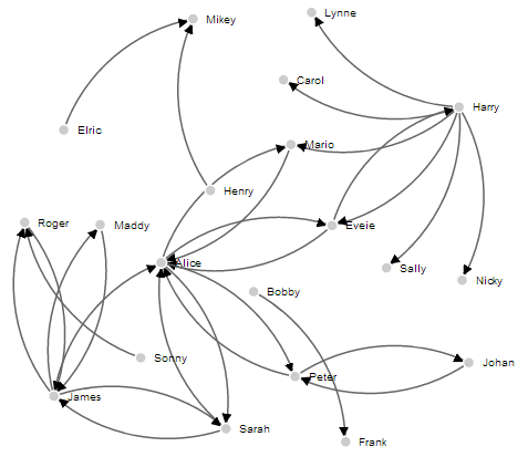
Here the charged nodes are trying to arrange themselves at an appropriate distance, but the length of the links means that their arrangement is not very pretty. Likewise if we change the value to 30 we get the following;

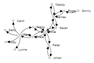
Here the link distance allows for a symmetrical layout, but the distance is too short to be practical.

.charge(-300) sets the force between nodes. Negative values of charge results in node repulsion, while a positive value results in node attraction. In our example, if we vary the value to 150 we get this result;

It’s not exactly easy to spot, but the graph feels a little ‘lazy’. The nodes don’t find their equilibrium easily or at all. Setting the value higher than 300 (for our example) keeps all the nodes nice and spread out, but where there are other separate discrete linked nodes (as there are in our example) they tend to get forced away from the centre of the defined area.

.on("tick", tick) runs the animation of the force layout one ‘step’. It’s this progression of steps that gives the force layout diagram it’s fluid movement.

.start(); Starts the simulation; this method must be called when the layout is first created.

The next block of our code is the standard section that sets up our svg container.

var svg = d3.select("body").append("svg")
    .attr("width", width)
    .attr("height", height);

The next block of our code is used to create our arrowhead marker. I will be the first to admit that it has entered a realm of svg expertise that I do not have and the amount of extra memory power I would need to accumulate to understand it sufficiently to explain won’t be occurring in the near future. Please accept my apologies and as a small token of my regret, accept the following links as an invitation to learn more: http://www.w3.org/TR/SVG/coords.html#ViewBoxAttribute and http://www.w3schools.com/svg/svg_reference.asp?. What is useful to note here is that we define the label for our marker as end. We will use this in the next section to reference the marker as an object. This particular section of the code caused me some small amount of angst. The problem being when I attempted to adjust the width of the link lines in conjunction with the value set in the data for the link, it would also adjust the stroke-width of the arrowhead marker. Then when I attempted to adjust for the positioning of the arrow on the path, I could never get the maths right. Eventually I decided to stop struggling against it and encode the value of the line in a couple of different ways. One as opacity using discrete boundaries and the other using variable line width, but with the arrowheads a common size. We will cover both those solutions in the coming sections.

svg.append("svg:defs").selectAll("marker")
    .data(["end"])
  .enter().append("svg:marker")    
    .attr("id", String)
    .attr("viewBox", "0 -5 10 10")
    .attr("refX", 15)
    .attr("refY", -1.5)
    .attr("markerWidth", 6)
    .attr("markerHeight", 6)
    .attr("orient", "auto")
  .append("svg:path")
    .attr("d", "M0,-5L10,0L0,5");

The .data(["end"]) line sets our tag for a future part of the script to find this block and draw the marker.

.attr("refX", 15) sets the offset of the arrow from the centre of the circle. While it is designated as the X offset, because the object is rotating, it doesn’t correspond to the x (left and right) axis of the screen. The same is true of the .attr("refY", -1.5) line.

The .attr("markerWidth", 6) and .attr("markerHeight", 6) lines set the bounding box for the marker. So varying these will vary the space available for the marker.

The next block of code adds in our links as paths and uses the #end marker to draw the arrowhead on the end of it.

var path = svg.append("svg:g").selectAll("path")
    .data(force.links())
  .enter().append("svg:path")
    .attr("class", "link")
    .attr("marker-end", "url(#end)");

Then we define what our nodes are going to be.

var node = svg.selectAll(".node")
    .data(force.nodes())
  .enter().append("g")
    .attr("class", "node")
    .call(force.drag);

This uses the nodes data and adds the .call(force.drag); function which allows the node to be dragged by the mouse.

The next block adds the nodes as an svg circle.

node.append("circle")
    .attr("r", 5);

And then we add the name of the node with a suitable offset.

node.append("text")
    .attr("x", 12)
    .attr("dy", ".35em")
    .text(function(d) { return d.name; });

The last block of JavaScript is the ticks function. This block is responsible for updating the graph and most interestingly drawing the curvy lines between nodes.

function tick() {
    path.attr("d", function(d) {
        var dx = d.target.x – d.source.x,
            dy = d.target.y – d.source.y,
            dr = Math.sqrt(dx * dx + dy * dy);
        return "M" + 
            d.source.x + "," + 
            d.source.y + "A" + 
            dr + "," + dr + " 0 0,1 " + 
            d.target.x + "," + 
            d.target.y;
    });

    node
        .attr("transform", function(d) { 
		    return "translate(" + d.x + "," + d.y + ")"; });
}

This is another example where there are some easily recognisable parts of the code that set the x and y points for the ends of each link (d.source.x, d.source.y for the start of the curve and d.target.x, d.target.y for the end of the curve) and a transformation for the node points, but the cleverness is in the combination of the math for the radius of the curve (dr = Math.sqrt(dx * dx + dy * dy);) and the formatting of the svg associated with it. This is sadly beyond the scope of what I can comfortable explain, so we will have to be content with “the magic happens here”.

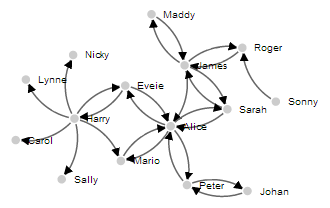
The end result should be a tidy graph that demonstrates nodes and directional links between them.

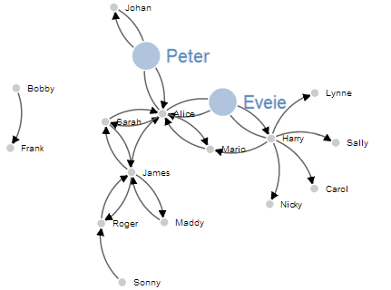
Directional Force Layout Diagram (Node Highlighting)

Following on from the Basic Force Layout Diagram, our next goal is to highlight our nodes so that we can get a better view of what ones they are (the view can get a little crowded as the nodes begin to increase in number).

To do this we are going to use a couple more of the mouse events that we first introduced in the tooltips section.

For this example we are going to use the click event (Triggered by a mouse click (mousedown and then mouseup over an element)) and the dblclick event (Triggered by two clicks within a short time over an element).

The single click will enlarge the node and the associated text and the double click will return the node and test to its original size.

The way to implement this is to first set a hook to capture when the event occurs, which calls a function which is laid out later in the script.

The hook is going to be part of the JavaScript where we define our nodes;

var node = svg.selectAll(".node")
    .data(force.nodes())
  .enter().append("g")
    .attr("class", "node")
    .on("click", click)        // Add in this line
    .on("dblclick", dblclick)  // Add in this line too
    .call(force.drag);

The two additional lines above tell the script that when it sees a click or a double-click on the node (since it’s part of the node set-up) to run either the click or dblclick functions.

The following two function blocks should be placed after the tick function but before the closing curly bracket and bracket as indicated;

function tick() {
    path.attr("d", function(d) {
        var dx = d.target.x – d.source.x,
            dy = d.target.y – d.source.y,
            dr = Math.sqrt(dx * dx + dy * dy);
        return "M" + 
            d.source.x + "," + 
            d.source.y + "A" + 
            dr + "," + dr + " 0 0,1 " + 
            d.target.x + "," + 
            d.target.y;
    });

    node
        .attr("transform", function(d) { 
		    return "translate(" + d.x + "," + d.y + ")"; });
}

        // <= Put the functions in here!

});

The click function is as follows;

function click() {
    d3.select(this).select("text").transition()
        .duration(750)
        .attr("x", 22)
        .style("fill", "steelblue")
        .style("stroke", "lightsteelblue")
        .style("stroke-width", ".5px")
        .style("font", "20px sans-serif");
    d3.select(this).select("circle").transition()
        .duration(750)
        .attr("r", 16)
        .style("fill", "lightsteelblue");
}

The first line declares the function name (click). Then we select the node that we’ve clicked on and then the associated text before we begin the declaration for our transition with the following;

d3.select(this).select("text").transition()

Then we define the new properties that will be in place after the transition. We move the text’s x position (.attr("x", 22)), make the text fill steel blue (.style("fill", "steelblue")), set the stroke around the edge of the text light steel blue (.style("stroke", "lightsteelblue")), set that stroke to half a pixel wide (.style("stroke-width", ".5px")) and increase the font size to 20 pixels (.style("font", "20px sans-serif");).

Then we do much the same for the circle component of the node. Select it, declare the transition, increase the radius and change the fill colour.

The dblclick function does exactly the same as the click function, but reverses the action to return the text and circle to the original settings.

function dblclick() {
    d3.select(this).select("circle").transition()
        .duration(750)
        .attr("r", 6)
        .style("fill", "#ccc");
    d3.select(this).select("text").transition()
        .duration(750)
        .attr("x", 12)
        .style("stroke", "none")
        .style("fill", "black")
        .style("stroke", "none")
        .style("font", "10px sans-serif");
}

The end result is a force layout diagram where you can click on nodes to increase their size (circle and text) and then double click to reset them if desired.

The full code for this diagram can be found on github or in the code samples bundled with this book (force-highlight.html and force.csv). A live example can be found on bl.ocks.org.

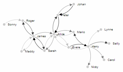
Directional Force Layout Diagram (varying link opacity)

The next variation to our force layout diagram is the addition of variation in the link to represent different values (think of the number of packets passed or the amount of money transferred).

There are a few different ways to do this, but by virtue of the inherent close linkages between the arrowhead marker and the link line, altering both in synchronicity proved to be beyond my meagre talents. However, I did find a couple of suitable alternatives and I will go through one here.

In this example we will take the value associated in the loaded data with the link and we will adjust the opacity of the link line in a staged way according to the range of values.

For example, in a range of link strengths from 0 to 100, the bottom 25% will be at opacity 0.25, from 25 to 50 will be 0.50, 50 to 75 will be 0.75 and above 75 will have an opacity of 1. So the final result looks a little like this;

The changes to the code to create this effect are focussed on creating an appropriate range for the values associated with the links and then applying the opacity according to that range in discrete steps.

The first change to the node highlighting code that we make is to the style section. The following elements are added;

path.link.twofive {
  opacity: 0.25;
}

path.link.fivezero {
  opacity: 0.50;
}

path.link.sevenfive {
  opacity: 0.75;
}

path.link.onezerozero {
  opacity: 1.0;
}

This provides our four different ‘classes’ of opacity.

Then in a block of code that comes just after the declaration of the force properties we have the following;

var	v = d3.scale.linear().range([0, 100]);

v.domain([0, d3.max(links, function(d) { return d.value; })]);

links.forEach(function(link) {
	if (v(link.value) <= 25) {
		link.type = "twofive";
	} else if (v(link.value) <= 50 && v(link.value) > 25) {
		link.type = "fivezero";
	} else if (v(link.value) <= 75 && v(link.value) > 50) {
		link.type = "sevenfive";
	} else if (v(link.value) <= 100 && v(link.value) > 75) {
		link.type = "onezerozero";
	}
});

Here we set the scale and the range for the variable v (var v = d3.scale.linear().range([0, 100]);). We then set the domain for v to go from 0 to the maximum value that we have in our link data.

The final block above uses a cascading set of if statements to assign a label to the type parameter of each link. This label is the linkage back to the styles we defined previously.

The final change is to take the line where we assigned a class of link to each link previously…

    .attr("class", "link")

…and add in our type parameter as well;

    .attr("class", function(d) { return "link " + d.type; })

Obviously if we wanted a greater number of opacity levels we would add in further style blocks (with the appropriate values) and modify our cascading if statements. I’m not convinced that this solution is very elegant for what I’m trying to do (it was a much better fit for the application that Mike Bostock applied it to originally where he designated different types of law suits) but I’ll take the result as a suitable way of demonstrating variation of value.

The full code for this diagram can be found on github or in the code samples bundled with this book (force-highlight-opacity.html and force.csv). A live example can be found on bl.ocks.org.

The full code for the Directional Force Layout Diagram with varying link opacity is also in the Appendix: Force Layout Diagram at the rear of the book.

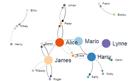
Directional Force Layout Diagram (Unique Node Colour)

The following example was put together in response to a question on the d3noob.org site from ‘Gino’. While the example isn’t precisely what Gino was wanting to achieve, it does illustrate the application of a colour palette to unique elements.

The end result looks like the following;

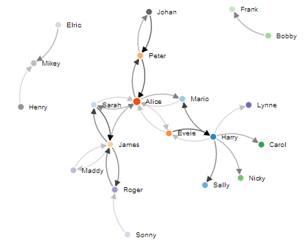
Here each of the nodes has had a separate colour applied to it from one of the 20 colour palette categorical colour ranges. An excellent overview of these ranges is on the d3 wiki.

The full code for this diagram can be found on github or in the code samples bundled with this book (force-colour-nodes.html and force.csv). A live example can be found on bl.ocks.org.

The changes required from the previous example with the altered opacity are pretty simple.

Firstly we declare the colour range we’re going to use in the variable section.

    color = d3.scale.category20c();

In this case we’ll use the category20c range.

Then we add the fill style for the circle to the code where we append the circles to our graphic.

node.append("circle")
    .attr("r", 5)
    .style("fill", function(d) { return color(d.name); });

The code applies the fill based on a function that returns a different colour based on each unique node name. So just to be clear here. We’re not setting a specific colour to a node. The colours are assigned as a function of where each name sits in the array of nodes (practically random, but in an ordered way :-)).

Then remove the style declarations in the function click() and function dblclick() where the fill colour is declared for the circles. This prevents the colours from turning grey or steelblue when they are clicked / double clicked. This means that we can click on a few of our new coloured nodes and their unique colours are retained thusly…

Good question Gino. Many thanks.