The Basics of Deep Learning
Deep learning is a subfield of machine learning that is concerned with the design and implementation of artificial neural networks (ANNs) with multiple layers, also known as deep neural networks (DNNs). These networks are inspired by the structure and function of the human brain, and are designed to learn from large amounts of data such as images, text, and audio.
A neural network consists of layers of interconnected nodes, or neurons, which are organized into an input layer, one or more hidden layers, and an output layer. Each neuron receives input from the neurons in the previous layer, performs a computation, and passes the result to the neurons in the next layer. The computation typically involves a dot product of the input with a set of weights and an activation function, which is a non-linear function applied to the result. The weights are the parameters of the network that are learned during training.
The basic building block of a deep neural network is an artificial neuron, also known as perceptron, which is a simple mathematical model for a biological neuron. A perceptron receives input from other neurons and it applies a linear transformation to the input, followed by a non-linear activation function.
Deep learning networks can be feedforward networks where the data flows in one direction from input to output, or recurrent networks where the data can flow in a cyclic fashion.
There are different types of deep learning architectures such as feedforward neural networks, convolutional neural networks (CNNs), recurrent neural networks (RNNs) and Generative Adversarial Networks (GANs). These architectures are designed to learn specific types of features and patterns from different types of data.
Deep learning models are trained using large amounts of labeled data, and typically use supervised or semi-supervised learning techniques. The training process involves adjusting the weights of the network to minimize a loss function, which measures the difference between the predicted output and the true output. This process is known as back-propagation, which is an algorithm for training the weights in a neural network by propagating the error back through the network. In the first AI book I wrote in the 1980s I covered the implementation of back-propagation in detail. As I write the material here on deep learning I think that it is more important for you to have the skills to choose appropriate tools for different applications and be less concerned about low-level implementation details. I think this characterizes the change in trajectory of AI from being about tool building to the skills of using available tools and sometimes previously trained models while spending more of your effort analyzing business functions and in general application domains.
Deep Learning has been applied to various fields such as Computer Vision, Natural Language Processing, Speech Recognition, etc.
Using TensorFlow.js for Building a Cancer Prediction Model
We will use TensorFlow.js on Node.js to build a neural network that classifies the same University of Wisconsin cancer dataset we used in the earlier chapter. This lets us directly compare the deep learning approach with the classic K-Nearest Neighbors classifier.
The examples for this chapter are in the directory source-code/deep_learning_basics.
The requirements for this chapter are:
1 npm install @tensorflow/tfjs-node
Why TensorFlow.js?
TensorFlow.js is Google’s official JavaScript/TypeScript deep learning framework. On Node.js with the @tensorflow/tfjs-node package, it provides:
- Native C++ backend: training and inference run through the same optimized TensorFlow C library used by Python TensorFlow.
- TypeScript-first API: full type definitions for the entire API surface.
- GPU support: optional GPU acceleration via
@tensorflow/tfjs-node-gpu. - Same API as Python: if you know TensorFlow/Keras in Python, the API is nearly identical.
Loading and Preparing the Data
We reuse the same CSV data files from our machine learning chapter. The data loading code parses the CSVs, scales the features, then wraps everything in TensorFlow tensors:
 1 import * as tf from "@tensorflow/tfjs-node";
 2 import { readFileSync } from "node:fs";
 3
 4 function loadData() {
 5   const parse = (p: string) => readFileSync(p, "utf-8").trim().split("\n").slice(1).map(l => l.split(",").map(Number));
 6   const train = parse("../machine-learning/labeled_cancer_data.csv");
 7   const test = parse("../machine-learning/labeled_test_data.csv");
 8   const [xTrain, yTrain] = [train.map(r => r.slice(0, 9)), train.map(r => [r[r.length - 1]])];
 9   const [xTest, yTest] = [test.map(r => r.slice(0, 9)), test.map(r => [r[r.length - 1]])];
10
11   const xT = tf.tensor2d(xTrain);
12   const mean = xT.mean(0), std = xT.sub(mean).square().mean(0).sqrt().add(tf.scalar(1e-8));
13   return {
14     xTrain: xT.sub(mean).div(std), yTrain: tf.tensor2d(yTrain),
15     xTest: tf.tensor2d(xTest).sub(mean).div(std), yTest: tf.tensor2d(yTest),
16     numTrain: xTrain.length, numTest: xTest.length, yTestRaw: yTest.map(r => r[0]),
17   };
18 }
Defining the Model
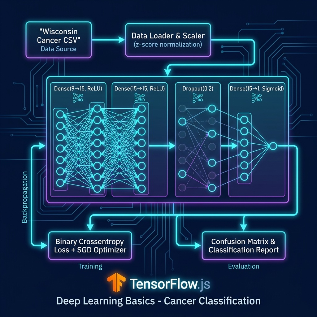
In TensorFlow.js, we define neural network architectures using the Sequential API. Our network has two hidden layers of 15 neurons with ReLU activation, a dropout layer for regularization, and a single output neuron:
1 function buildModel() {
2   const model = tf.sequential();
3   model.add(tf.layers.dense({ inputShape: [9], units: 15, activation: "relu" }));
4   model.add(tf.layers.dense({ units: 15, activation: "relu" }));
5   model.add(tf.layers.dropout({ rate: 0.2 }));
6   model.add(tf.layers.dense({ units: 1, activation: "sigmoid" }));
7   model.compile({ optimizer: tf.train.sgd(0.01), loss: "binaryCrossentropy", metrics: ["accuracy"] });
8   return model;
9 }
The Training Loop
TensorFlow.js handles training with the model.fit() method, which manages batching, gradient computation, and weight updates:
 1 console.log("\nTraining:");
 2 await model.fit(xTrain, yTrain, {
 3   epochs: 60, batchSize: 32, verbose: 0,
 4   callbacks: {
 5     onEpochEnd: (ep, logs) => {
 6       if ((ep + 1) % 10 === 0)
 7         console.log(`  Epoch ${String(ep + 1).padStart(3)}/60  loss: ${logs?.loss?.toFixed(4)}`);
 8     },
 9   },
10 });
Running the Example
Here is the complete output from running cancer_model.ts:
 1 $ tsx cancer_model.ts
 2 Training examples: 554
 3 Test examples:     15
 4
 5 Model Summary:
 6   Layer 1: Dense (9 → 15, ReLU)
 7   Layer 2: Dense (15 → 15, ReLU)
 8   Layer 3: Dropout (0.2)
 9   Layer 4: Dense (15 → 1, Sigmoid)
10
11 Training:
12   Epoch  10/60  loss: 0.6913
13   Epoch  20/60  loss: 0.6559
14   Epoch  30/60  loss: 0.6250
15   Epoch  40/60  loss: 0.5874
16   Epoch  50/60  loss: 0.5421
17   Epoch  60/60  loss: 0.4969
18
19 Confusion Matrix:
20 [[9, 0],
21  [1, 5]]
22
23 Classification Report:
24               precision    recall  f1-score   support
25          0.0       0.90      1.00      0.95         9
26          1.0       1.00      0.83      0.91         6
27     accuracy                           0.93        15
The model achieves 93% accuracy on the test set, matching the performance of our KNN classifier from the earlier chapter. The loss decreases steadily during training.
You can compare this TensorFlow.js example to our similar classification example using the KNN algorithm. The deep learning approach requires more code but gives us full control over the model architecture, training process, and the ability to scale to much larger and more complex problems.