“Classic” Machine Learning
“Classic” Machine Learning (ML) is a broad field that encompasses a variety of algorithms and techniques for learning from data. These techniques are used to make predictions, classify data, and uncover patterns and insights. Some of the most common types of classic ML algorithms include:
- Linear regression: a method for modeling the relationship between a dependent variable and one or more independent variables by fitting a linear equation to the observed data.
- Logistic regression: a method for modeling the relationship between a binary dependent variable and one or more independent variables by fitting a logistic function to the observed data.
- Decision Trees: a method for modeling decision rules based on the values of the input variables, which are organized in a tree-like structure.
- Random Forest: a method that creates multiple decision trees and averages the results to improve the overall performance of the model
- K-Nearest Neighbors (K-NN): a method for classifying data by finding the K-nearest examples in the training data and assigning the most similar common class among them.
- Naive Bayes: a method for classifying data based on Bayes’ theorem and the assumption of independence between the input variables.
We will be covering a very small subset of “classic” ML, and then dive deeper into Deep Learning in later chapters. Deep Learning differs from classic ML in several ways:
- Scale: Classic ML algorithms are typically designed to work with small to medium-sized datasets, while deep learning algorithms are designed to work with large-scale datasets, such as millions or billions of examples.
- Architecture: Classic ML algorithms have a relatively shallow architecture, with a small number of layers and parameters, while deep learning algorithms have a deep architecture, with many layers and millions or billions of parameters.
- Non-linearity: Classic ML algorithms are sometimes linear, (i.e., the relationship between the input and output is modeled by a linear equation), while deep learning algorithms are non-linear, (i.e., the relationship is modeled by a non-linear function).
- Feature extraction: “Classic” ML requires feature extraction, which is the process of transforming the raw input data into a set of features that can be used by the algorithm. Deep learning can automatically learn features from raw data, so it does not usually require too much separate effort for feature extraction.
So, Deep Learning is a subfield of machine learning that is focused on the design and implementation of artificial neural networks with many layers which are capable of learning from large-scale and complex data. It is characterized by its deep architecture, non-linearity, and ability to learn features from raw data, which sets it apart from “classic” machine learning algorithms.
Example Material
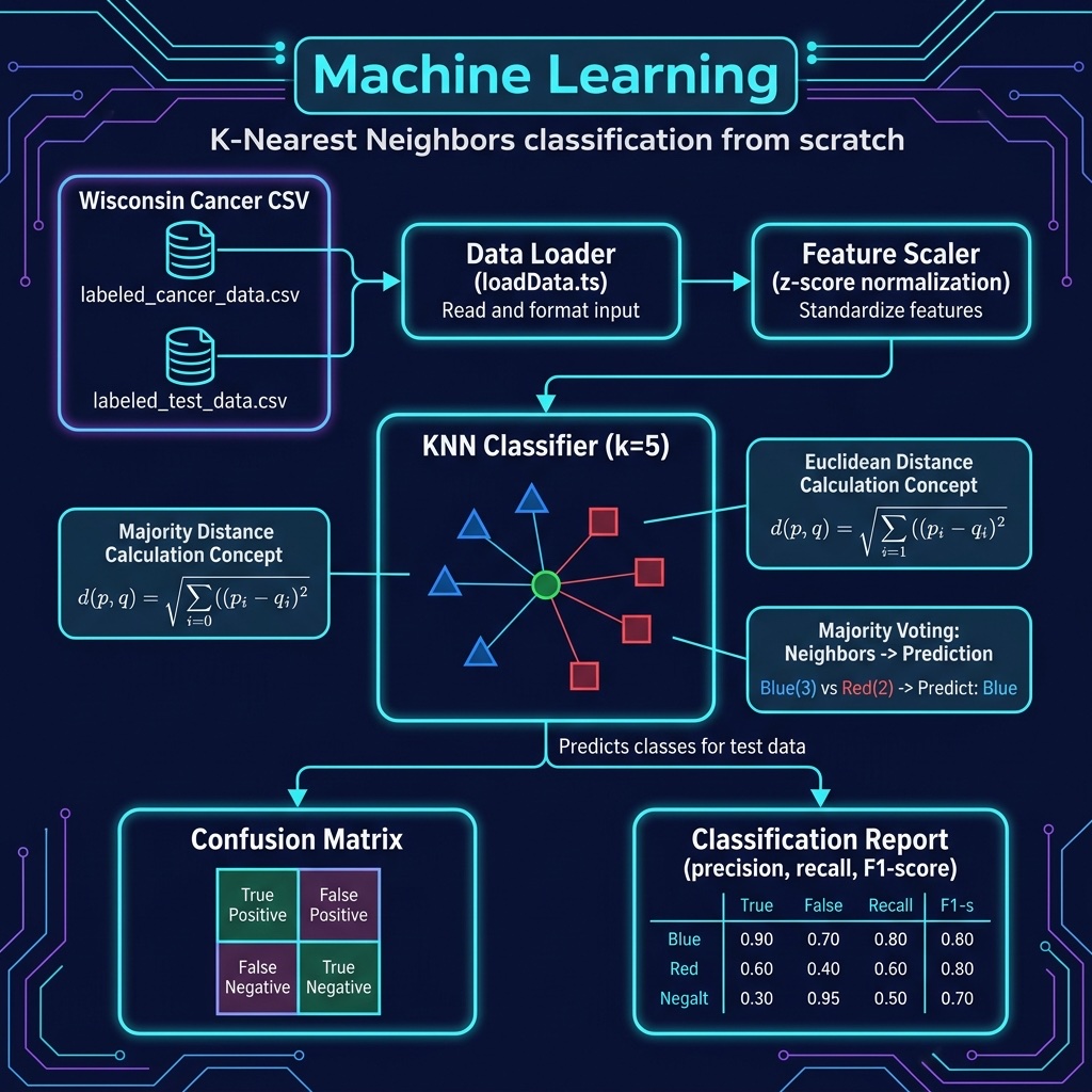
Here we cover a single example of what I think of as “classic machine learning”, a K-Nearest Neighbors classifier implemented from scratch in TypeScript. Later we cover deep learning in three separate chapters. Deep learning models are more general and powerful but it is important to recognize the types of problems that can be solved using the simpler techniques.
The only requirements for this chapter are Node.js and TypeScript, no external libraries needed. We implement KNN from scratch to demonstrate both the algorithm and TypeScript’s suitability for numerical computing.
The examples for this chapter are in the directory source-code/machine-learning.
Please note that the content in this book is heavily influenced by what I use in my own work. I mostly use deep learning so its coverage comprises half this book. For this classic machine learning chapter I only use a classification model. I will not be covering regression or clustering models.
We will use the same Wisconsin cancer dataset for both the following classification example and a deep learning classification example in a later chapter. Here are the first few rows of the file labeled_cancer_data.csv:
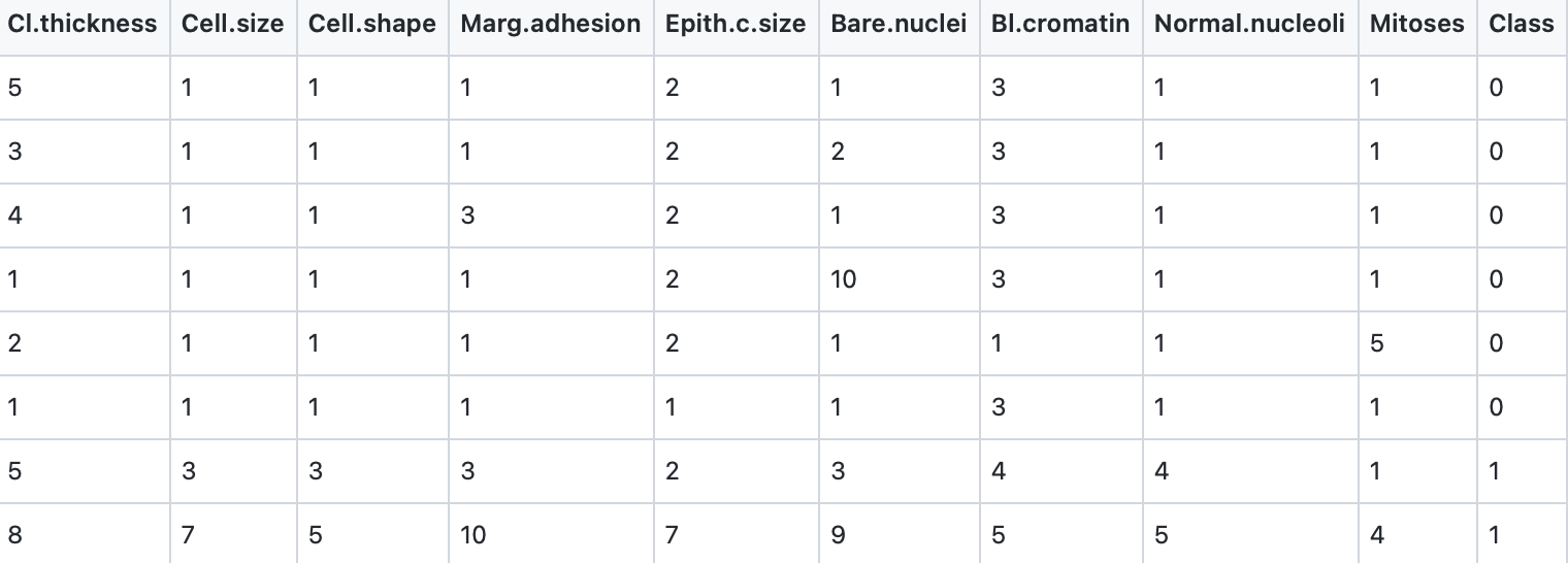
The last column class indicates the class of the sample, 0 for non-malignant and 1 for malignant.
Loading CSV Data
First, we need a utility to load our CSV data files. Unlike Python’s Pandas, we write a small CSV parser directly:
Listing of loadData.ts:
 1 import { readFileSync } from "node:fs";
 2
 3 export interface DataSet { xTrain: number[][]; yTrain: number[]; xTest: number[][]; yTest: number[] }
 4
 5 export function loadData(): DataSet {
 6   const parse = (p: string) => readFileSync(p, "utf-8").trim().split("\n").slice(1).map(l => l.split(",").map(Number));
 7   const [train, test] = ["labeled_cancer_data.csv", "labeled_test_data.csv"].map(parse);
 8   const split = (d: number[][]) => ({ x: d.map(r => r.slice(0, 9)), y: d.map(r => r[r.length - 1]) });
 9   const tr = split(train), te = split(test);
10   console.log(`Training: ${tr.x.length}  Test: ${te.x.length}`);
11   return { xTrain: tr.x, yTrain: tr.y, xTest: te.x, yTest: te.y };
12 }
We read the CSV file, skip the header row, and split each line by commas. In TypeScript we work with arrays of numbers directly rather than using a DataFrame abstraction.
Classification Using K-Nearest Neighbors
Classification is a type of supervised machine learning problem where the goal is to predict the class or category of an input sample based on a set of features. The goal of a classification model is to learn a mapping from the input features to the output class labels.
We implement the KNN algorithm from scratch. The key operations are: scale the features, compute Euclidean distances, find the K nearest neighbors, and take a majority vote.
 1 import { loadData } from "./loadData.js";
 2
 3 function fitScaler(data: number[][]) {
 4   const n = data.length, d = data[0].length;
 5   const means = new Array(d).fill(0), stds = new Array(d).fill(0);
 6   for (const row of data) for (let j = 0; j < d; j++) means[j] += row[j];
 7   for (let j = 0; j < d; j++) means[j] /= n;
 8   for (const row of data) for (let j = 0; j < d; j++) stds[j] += (row[j] - means[j]) ** 2;
 9   for (let j = 0; j < d; j++) stds[j] = Math.sqrt(stds[j] / n);
10   return { means, stds };
11 }
12
13 const applyScaler = (data: number[][], s: { means: number[]; stds: number[] }) =>
14   data.map(r => r.map((v, j) => s.stds[j] > 0 ? (v - s.means[j]) / s.stds[j] : 0));
15
16 const eucDist = (a: number[], b: number[]) =>
17   Math.sqrt(a.reduce((s, v, i) => s + (v - b[i]) ** 2, 0));
18
19 function knnPredict(trainX: number[][], trainY: number[], sample: number[], k: number): number {
20   const nearest = trainX.map((p, i) => ({ d: eucDist(sample, p), l: trainY[i] }))
21     .sort((a, b) => a.d - b.d).slice(0, k);
22   const votes: Record<number, number> = {};
23   for (const { l } of nearest) votes[l] = (votes[l] || 0) + 1;
24   return Number(Object.entries(votes).sort(([, a], [, b]) => b - a)[0][0]);
25 }
26
27 function classReport(actual: number[], predicted: number[]) {
28   console.log("              precision    recall  f1-score   support");
29   for (const cls of [0, 1]) {
30     const tp = actual.filter((a, i) => a === cls && predicted[i] === cls).length;
31     const fp = actual.filter((a, i) => a !== cls && predicted[i] === cls).length;
32     const fn = actual.filter((a, i) => a === cls && predicted[i] !== cls).length;
33     const sup = actual.filter(a => a === cls).length;
34     const pr = tp + fp > 0 ? tp / (tp + fp) : 0, re = tp + fn > 0 ? tp / (tp + fn) : 0;
35     const f1 = pr + re > 0 ? (2 * pr * re) / (pr + re) : 0;
36     console.log(`         ${cls.toFixed(1)}       ${pr.toFixed(2)}      ${re.toFixed(2)}      ${f1.toFixed(2)}         ${sup}`);
37   }
38   console.log(`    accuracy                           ${(actual.filter((a, i) => a === predicted[i]).length / actual.length).toFixed(2)}        ${actual.length}`);
39 }
40
41 const { xTrain, yTrain, xTest, yTest } = loadData();
42 const scaler = fitScaler(xTrain);
43 const xTrainS = applyScaler(xTrain, scaler), xTestS = applyScaler(xTest, scaler);
44 const yPred = xTestS.map(s => knnPredict(xTrainS, yTrain, s, 5));
45
46 const cm = [[0, 0], [0, 0]];
47 yTest.forEach((a, i) => cm[a][yPred[i]]++);
48 console.log(`\nConfusion Matrix:\n${cm.map(r => r.join("  ")).join("\n")}`);
49 console.log("\nClassification Report:");
50 classReport(yTest, yPred);
Note that we fit the scaler on the training data and then use the same fitted scaler to transform the test data. This is important: scaling the test data with parameters learned from the training set prevents data leakage and ensures a fair evaluation.
We can now train and test the model and evaluate how accurate the model is. In reading the following output, you should understand a few definitions. In machine learning, precision, recall, F1-score, and support are all metrics used to evaluate the performance of a classification model, specifically in regards to binary classification:
- Precision: the proportion of true positive predictions out of the total of all positive predictions made by the model. It is a measure of how many of the positive predictions were actually correct.
- Recall: the proportion of true positive predictions out of all actual positive observations in the data. It is a measure of how well the model is able to find all the positive observations.
- F1-score: the harmonic mean of precision and recall. It is a measure of the balance between precision and recall and is generally used when you want to seek a balance between precision and recall.
- Support: number of observations in each class.
These metrics provide an overall view of a model’s performance in terms of both correctly identifying positive observations and avoiding false positive predictions.
 1 $ tsx classification.ts
 2 Training: 554  Test: 15
 3
 4 Confusion Matrix:
 5 8  1
 6 0  6
 7
 8 Classification Report:
 9               precision    recall  f1-score   support
10          0.0       1.00      0.89      0.94         9
11          1.0       0.86      1.00      0.92         6
12     accuracy                           0.93        15
Classic Machine Learning Wrap-up
I have already admitted my personal biases in favor of deep learning over simpler machine learning and I proved that by implementing a single KNN classifier from scratch in this chapter. The advantage of TypeScript here is that the implementation is clear, type-safe, and requires zero external dependencies. In the next chapters we will use more sophisticated approaches.