Regression and Clustering
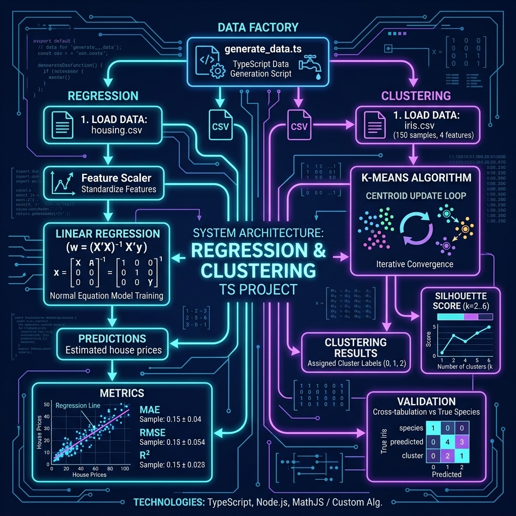
In the previous chapter we implemented a K-Nearest Neighbors classifier from scratch in TypeScript. Here we expand our coverage of “classic” machine learning with two more fundamental techniques: regression for predicting continuous values, and clustering for discovering groups in data without labeled targets.
No external libraries are required for this chapter, we implement everything from scratch in TypeScript.
The examples for this chapter are in the directory source-code/regression_and_clustering.
Regression: Predicting Housing Prices
Regression is a type of supervised machine learning where the goal is to predict a continuous numerical value rather than a class label. While classification asks “which category?”, regression asks “how much?” or “how many?”
Common regression algorithms include:
- Linear Regression: models the relationship between features and target as a straight line (or hyperplane in multiple dimensions).
- Polynomial Regression: extends linear regression by adding polynomial terms, allowing the model to capture non-linear relationships.
- Ridge and Lasso Regression: variants of linear regression that add regularization to prevent overfitting.
We will use a housing dataset (a subset of the California Housing dataset exported as CSV) with features describing census block groups (median income, average number of rooms, location, etc.), with the target being the median house value.
Linear Regression
Our first example fits a linear regression model using the normal equation, a closed-form solution that computes the optimal weights directly:
 1 import { readFileSync } from "node:fs";
 2
 3 type Matrix = number[][]; type Vector = number[];
 4
 5 const transpose = (m: Matrix): Matrix => m[0].map((_, i) => m.map(r => r[i]));
 6
 7 function matMul(a: Matrix, b: Matrix): Matrix {
 8   const [R, C, K] = [a.length, b[0].length, b.length];
 9   const r: Matrix = Array.from({ length: R }, () => new Array(C).fill(0));
10   for (let i = 0; i < R; i++) for (let j = 0; j < C; j++) for (let k = 0; k < K; k++) r[i][j] += a[i][k] * b[k][j];
11   return r;
12 }
13
14 function invertMatrix(m: Matrix): Matrix {
15   const n = m.length;
16   const aug: Matrix = m.map((row, i) => [...row, ...Array.from({ length: n }, (_, j) => i === j ? 1 : 0)]);
17   for (let i = 0; i < n; i++) {
18     let mx = i; for (let k = i + 1; k < n; k++) if (Math.abs(aug[k][i]) > Math.abs(aug[mx][i])) mx = k;
19     [aug[i], aug[mx]] = [aug[mx], aug[i]];
20     const p = aug[i][i]; if (Math.abs(p) < 1e-12) throw new Error("Singular matrix");
21     for (let j = 0; j < 2 * n; j++) aug[i][j] /= p;
22     for (let k = 0; k < n; k++) if (k !== i) { const f = aug[k][i]; for (let j = 0; j < 2 * n; j++) aug[k][j] -= f * aug[i][j]; }
23   }
24   return aug.map(r => r.slice(n));
25 }
26
27 function fitScaler(data: Matrix) {
28   const n = data.length, d = data[0].length;
29   const means = new Array(d).fill(0), stds = new Array(d).fill(0);
30   for (const r of data) for (let j = 0; j < d; j++) means[j] += r[j];
31   for (let j = 0; j < d; j++) means[j] /= n;
32   for (const r of data) for (let j = 0; j < d; j++) stds[j] += (r[j] - means[j]) ** 2;
33   for (let j = 0; j < d; j++) stds[j] = Math.sqrt(stds[j] / n);
34   return { means, stds };
35 }
36
37 const applyScaler = (data: Matrix, s: { means: Vector; stds: Vector }): Matrix =>
38   data.map(r => r.map((v, j) => s.stds[j] > 0 ? (v - s.means[j]) / s.stds[j] : 0));
39
40 function linearRegression(X: Matrix, y: Vector): Vector {
41   const Xb = X.map(r => [1, ...r]), Xt = transpose(Xb);
42   return matMul(invertMatrix(matMul(Xt, Xb)), matMul(Xt, y.map(v => [v]))).map(r => r[0]);
43 }
44
45 const predict = (X: Matrix, w: Vector): Vector =>
46   X.map(r => r.reduce((s, v, j) => s + w[j + 1] * v, w[0]));
47
48 const mae = (a: Vector, p: Vector) => a.reduce((s, v, i) => s + Math.abs(v - p[i]), 0) / a.length;
49 const rmse = (a: Vector, p: Vector) => Math.sqrt(a.reduce((s, v, i) => s + (v - p[i]) ** 2, 0) / a.length);
50 function r2Score(a: Vector, p: Vector) {
51   const m = a.reduce((x, y) => x + y, 0) / a.length;
52   return 1 - a.reduce((s, v, i) => s + (v - p[i]) ** 2, 0) / a.reduce((s, v) => s + (v - m) ** 2, 0);
53 }
54
55 // ---- Main ----
56 const content = readFileSync("housing.csv", "utf-8");
57 const lines = content.trim().split("\n");
58 const featureNames = lines[0].split(",").slice(0, -1);
59 const data = lines.slice(1).map(l => l.split(",").map(Number));
60 const X = data.map(r => r.slice(0, -1)), y = data.map(r => r[r.length - 1]);
61
62 const si = Math.floor(X.length * 0.8);
63 const scaler = fitScaler(X.slice(0, si));
64 const weights = linearRegression(applyScaler(X.slice(0, si), scaler), y.slice(0, si));
65 const yPred = predict(applyScaler(X.slice(si), scaler), weights);
66 const yTest = y.slice(si);
67
68 console.log(`Dataset: (${X.length}, ${X[0].length + 1})  Target: ${Math.min(...y).toFixed(2)} – ${Math.max(...y).toFixed(2)}`);
69 console.log(`\n=== Linear Regression Results ===`);
70 console.log(`  MAE: ${mae(yTest, yPred).toFixed(4)}  RMSE: ${rmse(yTest, yPred).toFixed(4)}  R²: ${r2Score(yTest, yPred).toFixed(4)}`);
71 console.log(`\nFeature coefficients (scaled):`);
72 featureNames.forEach((name, i) => {
73   const c = weights[i + 1];
74   console.log(`  ${name.padEnd(20)} ${c >= 0 ? "+" : ""}${c.toFixed(4)}`);
75 });
Because we scaled the features, the coefficients tell us the relative importance of each feature. MedInc (median income) typically has the largest positive coefficient, confirming that income is the strongest predictor of housing prices. The geographic features (Latitude and Longitude) are also very influential, location matters!
To evaluate a regression model, we use different metrics than classification:
- MAE (Mean Absolute Error): average magnitude of prediction errors in the same units as the target.
- RMSE (Root Mean Squared Error): like MAE but penalizes larger errors more heavily.
- R² (R-squared): the proportion of variance in the target explained by the model (1.0 = perfect, 0.0 = no better than predicting the mean).
Clustering: Discovering Groups in Data
Clustering is an unsupervised learning technique, unlike classification and regression, we do not provide labeled targets. Instead, the algorithm discovers natural groupings in the data.
K-Means is the most widely used clustering algorithm. It works by:
- Choosing K initial cluster centers (centroids).
- Assigning each data point to the nearest centroid.
- Recomputing each centroid as the mean of its assigned points.
- Repeating steps 2-3 until convergence.
We will use the classic Iris dataset (150 samples, 4 features measuring sepal and petal dimensions, with 3 known species). This lets us evaluate how well K-Means recovers the true species groupings.
K-Means Implementation
 1 import { readFileSync } from "node:fs";
 2
 3 function kMeans(data: number[][], k: number, maxIter = 100) {
 4   const n = data.length, d = data[0].length;
 5   const idx = new Set<number>();
 6   while (idx.size < k) idx.add(Math.floor(Math.random() * n));
 7   let centroids = [...idx].map(i => [...data[i]]);
 8   let labels = new Array(n).fill(0);
 9
10   for (let iter = 0; iter < maxIter; iter++) {
11     const newLabels = data.map(p => {
12       let minD = Infinity, best = 0;
13       for (let c = 0; c < k; c++) {
14         const dist = p.reduce((s, v, j) => s + (v - centroids[c][j]) ** 2, 0);
15         if (dist < minD) { minD = dist; best = c; }
16       }
17       return best;
18     });
19     if (newLabels.every((l, i) => l === labels[i])) break;
20     labels = newLabels;
21     centroids = Array.from({ length: k }, (_, c) => {
22       const members = data.filter((_, i) => labels[i] === c);
23       return members.length ? Array.from({ length: d }, (_, j) => members.reduce((s, p) => s + p[j], 0) / members.length) : centroids[c];
24     });
25   }
26   return { labels, centroids };
27 }
28
29 function silhouetteScore(data: number[][], labels: number[]): number {
30   const dist = (a: number[], b: number[]) => Math.sqrt(a.reduce((s, v, d) => s + (v - b[d]) ** 2, 0));
31   let total = 0;
32   for (let i = 0; i < data.length; i++) {
33     const same = data.filter((_, j) => j !== i && labels[j] === labels[i]);
34     const a = same.length > 0 ? same.reduce((s, p) => s + dist(data[i], p), 0) / same.length : 0;
35     const others = new Set(labels.filter(l => l !== labels[i]));
36     let b = Infinity;
37     for (const c of others) {
38       const m = data.filter((_, j) => labels[j] === c);
39       b = Math.min(b, m.reduce((s, p) => s + dist(data[i], p), 0) / m.length);
40     }
41     if (b === Infinity) b = 0;
42     total += b > a ? (b - a) / b : a > b ? (b - a) / a : 0;
43   }
44   return total / data.length;
45 }
Running the Clustering Example
 1 $ tsx clustering.ts
 2 Dataset: 150 samples, 4 features
 3 Features: ['sepal length', 'sepal width', 'petal length', 'petal width']
 4 Known species: ['setosa', 'versicolor', 'virginica']
 5
 6 === Silhouette Scores for Different k Values ===
 7   k=2: silhouette score = 0.5818
 8   k=3: silhouette score = 0.4599
 9   k=4: silhouette score = 0.3869
10   k=5: silhouette score = 0.3459
11   k=6: silhouette score = 0.3171
The silhouette score is highest at k=2, which suggests that the data most naturally splits into two groups. This makes biological sense: setosa is very distinct from the other two species, while versicolor and virginica overlap considerably.
Regression and Clustering Wrap-up
In this chapter we covered two fundamental machine learning techniques beyond classification:
- Regression lets us predict continuous values. We saw that even simple linear regression can be informative, and that feature coefficients reveal which inputs drive predictions.
- Clustering discovers structure in unlabeled data. We used silhouette scores to evaluate cluster quality and cross-tabulations to compare clusters against known labels.
Together with the classification example in the previous chapter, you now have hands-on experience with the three core tasks of classic machine learning, all implemented from scratch in TypeScript. In the next chapter we will explore the data preparation work that comes before training any model.
Optional Practice Problems
-
Ridge Regression (L2 Regularization): The current linear regression implementation in regression.ts uses the normal equation:

In practice, if features are highly correlated (collinear) or data is scarce,
 may be close to singular, causing numerical instability. Ridge regression addresses this by adding a regularization penalty
  to the diagonal of before inversion:
where
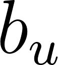 is the identity matrix (typically leaving the bias term weight
 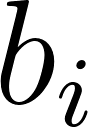 unregularized). Modify the
 linearRegressionfunction to support Ridge regression. Experiment with different values (e.g., 0.1,1.0,10.0) and compare the resulting test metrics (MAE, RMSE, ) and the magnitude of the feature coefficients.
 -
Gradient Descent Solver: Calculating the normal equation directly requires computing a matrix inversion, which scales as
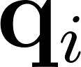 with the number of features
  . For high-dimensional datasets, Gradient Descent is a more scalable alternative. Implement linear regression using gradient descent:
- Implement a function
linearRegressionGD(X: Matrix, y: Vector, learningRate: number, epochs: number): Vectorthat iteratively updates the model weights to minimize Mean Squared Error (MSE). - Test your solver on the housing dataset and compare the final weights and training time with the closed-form normal equation solver.
-
K-Means++ Initialization: The K-Means implementation in clustering.ts initializes centroids by choosing
 random samples. This simple approach can lead to sub-optimal local minima depending on the initialization. The K-Means++ algorithm selects the first centroid at random, and then selects subsequent centroids with a probability proportional to their squared distance to the nearest existing centroid.
- Implement K-Means++ initialization.
- Compare the average number of iterations required to converge and the average silhouette scores achieved using K-Means++ versus random initialization over 50 runs.
-
Alternative Distance Metrics for K-Means: The current clustering implementation uses squared Euclidean distance to assign points to centroids. In some domains, alternative metrics like Manhattan distance (
 norm) or Cosine distance are more effective.
- Refactor the
kMeansfunction to accept a customizable distance function. - Implement Manhattan distance and Cosine distance.
- Run the clustering algorithm with these metrics on the Iris dataset and compare their resulting cluster assignments and silhouette scores against Euclidean distance.