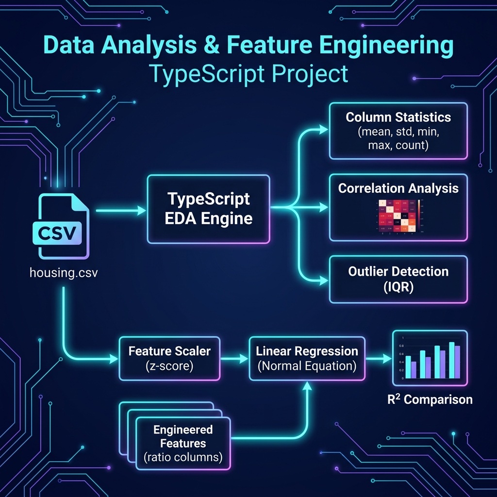
Exploratory Data Analysis and Feature Engineering
Before training any machine learning model, you need to understand your data. Exploratory Data Analysis (EDA) is the process of examining a dataset to summarize its main characteristics, find patterns, detect anomalies, and check assumptions. Feature engineering is the art of creating new input variables, or transforming existing ones, to improve model performance.
These steps often make the difference between a mediocre model and a good one. As the saying goes: “garbage in, garbage out.”
No external libraries are required for this chapter, we work with TypeScript arrays and our own utility functions.
The examples for this chapter are in the directory source-code/data_analysis_and_feature_engineering.
We continue using the California Housing dataset from a previous chapter.
Exploratory Data Analysis
Loading and Inspecting the Data
The first thing to do with any dataset is to understand its shape, types, and basic statistics:
 1 import { readFileSync } from "node:fs";
 2
 3 function loadCSV(path: string) {
 4   const lines = readFileSync(path, "utf-8").trim().split("\n");
 5   return { headers: lines[0].split(",").map(h => h.trim()), data: lines.slice(1).map(l => l.split(",").map(Number)) };
 6 }
 7
 8 const { headers, data } = loadCSV("housing.csv");
 9 console.log(`=== Dataset Overview ===\nShape: ${data.length} rows × ${headers.length} columns\n\nColumns:`);
10 headers.forEach(h => console.log(`  ${h}`));
Running our eda.ts script gives us:
 1 $ tsx eda.ts
 2 === Dataset Overview ===
 3 Shape: 20640 rows × 9 columns
 4
 5 Columns:
 6   MedInc
 7   HouseAge
 8   AveRooms
 9   AveBedrms
10   Population
11   AveOccup
12   Latitude
13   Longitude
14   MedHouseVal
Summary Statistics
 1 function columnStats(data: number[][], i: number) {
 2   const col = data.map(r => r[i]), n = col.length;
 3   const mean = col.reduce((a, b) => a + b, 0) / n;
 4   const std = Math.sqrt(col.reduce((s, x) => s + (x - mean) ** 2, 0) / n);
 5   return { n, mean, std, min: Math.min(...col), max: Math.max(...col) };
 6 }
 7
 8 console.log("\n=== Summary Statistics ===");
 9 headers.forEach((name, i) => {
10   const s = columnStats(data, i);
11   console.log(`  ${name.padEnd(15)} mean=${s.mean.toFixed(2).padStart(8)} std=${s.std.toFixed(2).padStart(8)} min=${s.min.toFixed(2).padStart(8)} max=${s.max.toFixed(2).padStart(8)}`);
12 });
Notice the wide range differences: Population ranges from 3 to 35,682 while AveBedrms ranges from 0.33 to 34.07. This tells us we will need feature scaling before training most models.
Correlation Analysis
Understanding which features correlate with the target helps guide feature selection and engineering:
 1 function correlation(x: number[], y: number[]): number {
 2   const mx = x.reduce((a, b) => a + b, 0) / x.length;
 3   const my = y.reduce((a, b) => a + b, 0) / y.length;
 4   let num = 0, dx = 0, dy = 0;
 5   for (let i = 0; i < x.length; i++) { num += (x[i] - mx) * (y[i] - my); dx += (x[i] - mx) ** 2; dy += (y[i] - my) ** 2; }
 6   return dx > 0 && dy > 0 ? num / Math.sqrt(dx * dy) : 0;
 7 }
 8
 9 const targetIdx = headers.indexOf("MedHouseVal");
10 const target = data.map(r => r[targetIdx]);
11
12 console.log("\n=== Correlation with MedHouseVal ===");
13 headers.map((name, i) => ({ name, corr: i !== targetIdx ? correlation(data.map(r => r[i]), target) : 0 }))
14   .filter(c => c.name !== "MedHouseVal")
15   .sort((a, b) => Math.abs(b.corr) - Math.abs(a.corr))
16   .forEach(({ name, corr }) => console.log(`  ${name.padEnd(22)} ${corr >= 0 ? "+" : ""}${corr.toFixed(4)}`));
MedInc (median income) stands out with a correlation of +0.69, by far the strongest predictor. This aligns with what we saw from the regression coefficients in the previous chapter.
Outlier Detection
The IQR (Interquartile Range) method flags values that fall more than 1.5 × IQR below Q1 or above Q3:
 1 function countOutliers(values: number[]): number {
 2   const sorted = [...values].sort((a, b) => a - b);
 3   const q1 = sorted[Math.floor(sorted.length * 0.25)];
 4   const q3 = sorted[Math.floor(sorted.length * 0.75)];
 5   const iqr = q3 - q1;
 6   return values.filter(v => v < q1 - 1.5 * iqr || v > q3 + 1.5 * iqr).length;
 7 }
 8
 9 console.log("\n=== Outlier Counts (IQR method) ===");
10 headers.forEach((name, i) => {
11   const out = countOutliers(data.map(r => r[i]));
12   console.log(`  ${name.padEnd(22)} ${out} outliers (${((out / data.length) * 100).toFixed(1)}%)`);
13 });
Feature Engineering
Feature engineering is where domain knowledge meets data science. By creating new features that better represent the underlying patterns, we can significantly improve model performance, sometimes more than choosing a fancier algorithm.
Creating New Features
We can derive meaningful features by combining existing ones:
 1 // Indices for the features we need
 2 const roomsIdx = headers.indexOf("AveRooms");
 3 const bedrmIdx = headers.indexOf("AveBedrms");
 4 const occupIdx = headers.indexOf("AveOccup");
 5 const ageIdx = headers.indexOf("HouseAge");
 6 const popIdx = headers.indexOf("Population");
 7
 8 const engineered = data.map(row => [
 9   ...row.slice(0, -1),  // original features (excluding target)
10   row[roomsIdx] / (row[occupIdx] || 1),    // RoomsPerHousehold
11   row[bedrmIdx] / (row[roomsIdx] || 1),    // BedroomRatio
12   row[popIdx] / (row[ageIdx] || 1),         // PopPerHousehold
13 ]);
- RoomsPerHousehold: a proxy for house size relative to occupancy.
- BedroomRatio: what fraction of rooms are bedrooms (a measure of house layout).
- PopPerHousehold: population growth rate proxy (newer areas with high population).
Handling Missing Data
Real datasets almost always have missing values. Common strategies include:
- Drop rows: simple but loses data.
- Fill with mean/median: preserves dataset size; median is more robust to outliers.
- Fill with a model prediction: more sophisticated but adds complexity.
1 function fillMissing(values: number[]): number[] {
2   const valid = values.filter(v => !isNaN(v));
3   const sorted = [...valid].sort((a, b) => a - b);
4   const median = sorted[Math.floor(sorted.length / 2)];
5   return values.map(v => isNaN(v) ? median : v);
6 }
Measuring the Impact
The ultimate test of feature engineering is whether it improves model performance. We compare a Linear Regression model with the original 8 features against one with our 11 engineered features:
1 === Model Comparison: Original vs. Engineered Features ===
2   Original (8 features)           R² = 0.5758
3   Engineered (11 features)        R² = 0.6622
Our engineered features improved R² from 0.58 to 0.66, a 15% improvement in explained variance, using the exact same algorithm. This demonstrates why feature engineering is often more valuable than model selection for improving results.
EDA and Feature Engineering Wrap-up
In this chapter we covered the essential data preparation skills that precede model training:
- EDA helps you understand your data through summary statistics, correlation analysis, and outlier detection. Never skip this step.
- Feature engineering transforms raw data into more informative inputs: creating derived features, encoding categories, handling missing values, and scaling.
- The payoff is real: our engineered features produced a 15% improvement in model performance with zero algorithm changes.
These techniques apply to every machine learning project, whether you are using classic algorithms or deep learning frameworks. In the next part of this book, we move into deep learning.