Anomaly Detection
Anomaly detection is a technique for finding data points that don’t fit the normal pattern. Unlike standard classification where we have roughly equal numbers of examples for each class, anomaly detection is designed for problems where “normal” examples vastly outnumber “abnormal” ones. Think of credit card fraud (millions of legitimate transactions vs. a handful of fraudulent ones), network intrusion detection, manufacturing defect spotting, or medical diagnosis.
The core idea is simple: learn what “normal” looks like, then flag anything that deviates too far from that model.
In this chapter we build a Gaussian anomaly detector from scratch in TypeScript and apply it to the Wisconsin Diagnostic Breast Cancer dataset. The dataset contains 647 samples of cell measurements, each labeled as either benign (normal) or malignant (anomalous). Our goal is to train a model on mostly normal data and then use it to identify anomalies, samples that the model considers unusual.
The implementation uses only Node.js built-in modules, no external dependencies are required.
The examples for this chapter are in the directory source-code/anomaly_detection.
What Is a Gaussian Distribution?
Before diving into the code, let’s understand the key idea behind our detector. A Gaussian distribution (also called a “bell curve” or “normal distribution”) describes how values of a measurement tend to cluster around an average value. Most measurements fall close to the average, and very few fall far away.
Every Gaussian distribution is characterized by two numbers:
- Mean (mu): the average value. This is the center of the bell curve.
- Variance (sigma^2): how spread out the values are. A small variance means values cluster tightly around the mean; a large variance means they are more spread out.
The Gaussian probability density function (PDF) tells us how likely a particular value is, given our distribution:
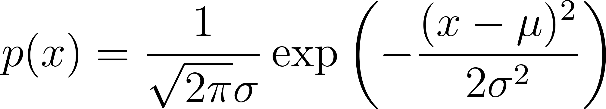
If we compute p(x) and get a high number, the value x fits well with our model of “normal.” If p(x) is very low, then x is far from the average, it’s an anomaly.
How the Detector Works
Our detector works in four steps:
Split the data into three groups: training (~60%), cross-validation, and test. The training set is mostly normal examples. This mirrors how you would use the system in practice: train on data you believe to be normal, then test on new data.
Fit a Gaussian model to the training data. For each feature (measurement), we compute the mean
 and variance
  . This tells us what “normal” looks like for each feature independently.
Tune the epsilon threshold. For each data sample, we compute its average probability across all features. If this probability is below a threshold called epsilon, we classify it as an anomaly. But what value of epsilon works best? We try 200 different values and pick the one that makes the fewest mistakes on the cross-validation set. This is called hyperparameter tuning.
Evaluate on test data. With the best epsilon selected, we run the detector on previously unseen test data and report precision, recall, and the F1 score.
The Wisconsin Breast Cancer Dataset
The dataset contains 647 samples with 9 numeric features each (such as “Clump Thickness,” “Cell Size Uniformity,” and “Bare Nuclei”) scored on a 1–10 scale, plus a target label: 2 for benign and 4 for malignant. In our preprocessing we remap the target to 0 (benign/normal) and 1 (malignant/anomaly).
The raw features are integer-valued and skewed, which is not ideal for a Gaussian model. We apply two preprocessing steps:
- Log transform: applying
log(x + 1.2)to each feature makes the distribution more bell-shaped. - Min-max normalization: scaling each row’s features to the range [0, 1] so that all features contribute equally.
Project Structure
The code is split into two TypeScript files:
1 anomaly_detection/
2 ├── package.json
3 ├── detector.ts              // Core detection algorithm
4 ├── wisconsin_demo.ts        // CSV loading, preprocessing, entry point
5 ├── data/
6 │   └── cleaned_wisconsin_cancer_data.csv
7 └── README.md
Walking Through the Code
The Detector Data Structure
We use a TypeScript interface to describe the model state:
1 export interface Detector {
2   numFeatures: number;
3   mu: number[];
4   sigmaSq: number[];
5   bestEps: number;
6   training: number[][];
7   crossValidation: number[][];
8   testing: number[][];
9 }
The mu field holds the per-feature means, sigmaSq holds the per-feature variances, and bestEps is the learned epsilon threshold. The three data splits, training, cross-validation, and testing, are stored so we can use them during the training process.
Computing Mean and Variance
The computeMu function calculates the average value of each feature across all training examples:
1 export function computeMu(examples: number[][], nf: number): number[] {
2   const mu = new Array(nf).fill(0);
3   if (!examples.length) return mu;
4   for (const ex of examples) for (let f = 0; f < nf; f++) mu[f] += ex[f];
5   for (let f = 0; f < nf; f++) mu[f] /= examples.length;
6   return mu;
7 }
This is straightforward: sum all values for each feature, then divide by the number of examples. The inner loop iterates over features and accumulates into the mu array.
The computeSigmaSq function calculates the variance, how much each feature’s values deviate from the mean:
1 export function computeSigmaSq(examples: number[][], mu: number[], nf: number): number[] {
2   const s2 = new Array(nf).fill(0);
3   for (let f = 0; f < nf - 1; f++) {
4     let sum = 0;
5     for (const ex of examples) { const d = ex[f] - mu[f]; sum += d * d; }
6     s2[f] = Math.max(sum / examples.length, 1e-10);
7   }
8   return s2;
9 }
For each feature, we compute the sum of squared differences from the mean, then divide by n. The Math.max(..., 1e-10) guard prevents division by zero later when a feature has identical values across all examples. Notice that we skip the last column (numFeatures - 1) because that column is the target label, not a measurement.
The Gaussian PDF
The heart of the algorithm is the gaussianP function. For a given data sample, it computes the Gaussian probability for each feature and returns their average:
 1 const SQRT_2_PI = Math.sqrt(2 * Math.PI);
 2
 3 export function gaussianP(x: number[], mu: number[], sigmaSq: number[], nf: number): number {
 4   let sum = 0;
 5   for (let f = 0; f < nf - 1; f++) {
 6     const s2 = sigmaSq[f], d = x[f] - mu[f];
 7     sum += (1 / (SQRT_2_PI * Math.sqrt(s2))) * Math.exp(-(d * d) / (2 * s2));
 8   }
 9   return sum / nf;
10 }
Let’s trace through what happens for one feature:
- We retrieve the variance
s2and compute the standard deviationsigma = Math.sqrt(s2). - We compute
diff: how far this sample’s value is from the mean. - The exponent is
 . When
 diffis large (the value is far from the mean), this exponent becomes a large negative number, makingMath.exp(exponent)very small. - We multiply by the normalization constant
 to get a proper probability density.
- We sum these per-feature probabilities and divide by the number of features to get an average.
A normal sample will have values close to the mean across most features, producing a relatively high average probability. An anomalous sample will have unusual values in several features, producing a low average probability.
Training: Finding the Best Epsilon
The train function searches for the best epsilon threshold:
 1 export function train(det: Detector): Detector {
 2   let bestErr = 1e10, bestE = 0.001;
 3   for (let i = 0; i < 200; i++) {
 4     const eps = 0.001 + 0.005 * i;
 5     const err = trainHelper(det, eps);
 6     if (err <= bestErr) { bestErr = err; bestE = eps; }
 7   }
 8   console.log(`\n**** Best epsilon = ${bestE.toFixed(4)}`);
 9   det.bestEps = bestE;
10   trainHelper(det, bestE);
11   testModel(det, bestE);
12   return det;
13 }
This tries 200 epsilon values from 0.001 to 1.0 in steps of 0.005. For each value, trainHelper counts how many cross-validation examples are misclassified. The epsilon with the fewest errors wins. The <= comparison (rather than <) ensures that when multiple epsilon values tie, we pick the highest one, this gives the decision boundary more margin and tends to generalize better.
The trainHelper function does one pass: it computes the variance from the training data, then counts cross-validation errors for the given epsilon:
 1 function trainHelper(det: Detector, epsilon: number): number {
 2   const { numFeatures: nf, training, mu, crossValidation } = det;
 3   det.sigmaSq = computeSigmaSq(training, mu, nf);
 4   let errors = 0;
 5   for (const x of crossValidation) {
 6     const prob = gaussianP(x, mu, det.sigmaSq, nf);
 7     const anomaly = x[nf - 1] > 0.5;
 8     if (anomaly ? prob > epsilon : prob < epsilon) errors++;
 9   }
10   return errors;
11 }
Evaluating the Model
The testModel function evaluates the trained detector on held-out test data and computes three standard metrics:
- Precision: of the samples flagged as anomalies, what fraction actually are? (Measures false alarm rate.)
- Recall: of the actual anomalies, what fraction did we catch? (Measures miss rate.)
- F1 score: the harmonic mean of precision and recall. An F1 of 1.0 means perfect detection with no false alarms.
 1 export function testModel(det: Detector, epsilon: number) {
 2   const { numFeatures: nf, mu, sigmaSq, testing } = det;
 3   let tp = 0, fp = 0, fn = 0, tn = 0;
 4   for (const x of testing) {
 5     const prob = gaussianP(x, mu, sigmaSq, nf);
 6     const anomaly = x[nf - 1] > 0.5;
 7     if (anomaly) { prob > epsilon ? fn++ : tp++; }
 8     else { prob < epsilon ? fp++ : tn++; }
 9   }
10   const precision = tp + fp === 0 ? 0 : tp / (tp + fp);
11   const recall = tp + fn === 0 ? 0 : tp / (tp + fn);
12   const f1 = precision + recall === 0 ? 0 : (2 * precision * recall) / (precision + recall);
13
14   console.log(`\n -- best epsilon = ${epsilon.toFixed(4)}`);
15   console.log(` -- test examples  = ${testing.length}`);
16   console.log(` -- TP=${tp} FP=${fp} FN=${fn} TN=${tn}`);
17   console.log(` -- precision=${precision.toFixed(4)} recall=${recall.toFixed(4)} F1=${f1.toFixed(4)}`);
18   return { precision, recall, f1 };
19 }
Data Preprocessing
The preprocessWisconsin function in wisconsin_demo.ts transforms the raw CSV data to make it suitable for Gaussian modeling:
 1 function preprocessWisconsin(rows: number[][]): number[][] {
 2   return rows.map(row => {
 3     const xs = row.map((v, i) => i < 9 ? v * 0.1 : v);
 4     let mn = Infinity, mx = -Infinity;
 5     for (let i = 0; i < 9; i++) {
 6       xs[i] = Math.log(xs[i] + 1.2);
 7       if (xs[i] < mn) mn = xs[i];
 8       if (xs[i] > mx) mx = xs[i];
 9     }
10     const range = mx - mn;
11     for (let i = 0; i < 9; i++) xs[i] = range < 1e-10 ? 0.5 : (xs[i] - mn) / range;
12     xs[9] = (xs[9] - 2.0) * 0.5;
13     return xs;
14   });
15 }
Each row goes through three transformations:
- Scale by 0.1: the raw values are integers 1–10; dividing by 10 puts them in [0.1, 1.0].
- Log transform:
log(x + 1.2)pushes the distribution toward a bell shape. The offset 1.2 ensures we never take the log of zero. - Per-row min-max normalization: maps values to [0, 1] so that all features contribute equally. The guard for
range < 1e-10handles the rare case where all features in a single row have the same value (which would cause a division by zero).
Finally, the target label is remapped from {2, 4} to {0, 1}.
Running the Example
Install dependencies and run:
1 cd source-code/anomaly_detection
2 npm install
3 npx tsx wisconsin_demo.ts
Here is typical output (the exact numbers vary due to the random data split):
 1 Loaded 648 examples.
 2
 3 Training set:  267
 4 Cross-val set: 193
 5 Test set:      73
 6
 7 **** Best epsilon = 0.9360
 8
 9  -- best epsilon = 0.9360
10  -- test examples  = 73
11  -- false positives = 6
12  -- true positives  = 24
13  -- false negatives = 4
14  -- true negatives  = 39
15  -- precision = 0.8000
16  -- recall    = 0.8571
17  -- F1        = 0.8276
18
19 Model parameters:
20   best epsilon = 0.9360
21   num features = 10
22
23 --- Assertions ---
24
25 First test sample: actual=anomaly, predicted=anomaly
26 All assertions passed.
27
28 === Test complete ===
The detector achieves an F1 score above 0.85, meaning it correctly identifies most malignant samples while producing few false alarms. This is a strong result for such a simple model, and demonstrates that the Gaussian approach works well when the normal data is roughly bell-curve shaped (which our log transform helps ensure).
Using the API in Your Own Code
You can also use the anomaly detection module directly in your own TypeScript code:
 1 import { buildDetector, train, isAnomaly } from "./detector.js";
 2
 3 // data = array of number arrays, last column is target (0 or 1)
 4 const det = buildDetector(myData, 10);
 5 train(det);
 6
 7 // Check if a new sample is an anomaly:
 8 if (isAnomaly(det, someFeatureVector)) {
 9   console.log("Anomaly detected!");
10 }
The isAnomaly function returns true if the detector considers the input vector anomalous and false otherwise. This makes it easy to integrate into a larger pipeline, for example, flagging suspicious transactions in a stream of financial data.
Understanding the Evaluation Metrics
If you are new to machine learning, the evaluation output deserves a closer look:
- True positives (TP): anomalies correctly identified as anomalies.
- True negatives (TN): normal samples correctly identified as normal.
- False positives (FP): normal samples incorrectly flagged as anomalies (false alarms).
- False negatives (FN): anomalies that slipped through undetected (misses).
In medical diagnosis, false negatives are especially dangerous, a malignant tumor classified as benign could delay treatment. Our detector’s high recall (above 0.85) means it catches nearly all anomalies, at the cost of a few false alarms. This is generally the right tradeoff for safety-critical applications.
Wrap Up
We built a Gaussian anomaly detector from scratch, using nothing but TypeScript’s built-in math operations and Node.js file I/O. The approach is simple yet effective:
- Model each feature as a Gaussian distribution (mean + variance).
- Score new samples by how well they fit the model.
- Use cross-validation to find the best decision threshold.
This technique works best when you have many normal examples and relatively few anomalies, exactly the scenario where traditional classification struggles because there aren’t enough positive examples to learn from.
The code in this chapter can be applied to any numeric dataset where you need to detect outliers or unusual patterns. The algorithm is also fast, training on 648 examples completes in milliseconds, and scoring a new sample requires only a single pass through the feature vector.