Leanpub: Publish Early, Publish Often

Custom Exporters

As much as the available information from node_exporter is extraordinary, if you have developed a project or need to monitoring something unique, you will want to integrate it with Prometheus / Grafana. This is where custom exporters come in.

The process is described as ‘instrumentation’. In the sense that it’s like adding sensors to different parts of your system that will report back the data your looking for. The same way developers of high performance vehicles will add measuring instruments to gauge performance.

We can add this instrumentation via client libraries that are supported by Prometheus or from a range of third party libraries. The officially supported libraries are;

Go
Java or Scala
Python
Ruby

When implemented they will gather the information and expose it via a HTTP endpoint (the same way that node_exporter does with http://<IP Address>:9100/metrics.

In the example that we will develop we will collect information from a platform that is measuring the depth of water in a tank and the temperature of the water and we will use the Python client library. Readers of some of my other books may recognise that as the data that I describe measuring in Raspberry Pi Computing: Ultrasonic Distance Measurement and Raspberry Pi Computing: Temperature Measurement.

Metrics

We could easily cut straight to the code and get measuring, (and feel free to do that if you would prefer) but it would be useful to learn a little about the different metric types available and some of the ways that they should be implemented to make the end result integrate with other metrics and follow best practices for flexibility and efficiency.

Metric Types

Prometheus recognises four different core metric types;

Counter: Where the value of the metric increments
Gauge: Where the metric value can increase or decrease
Histogram: Where values are summed into configurable ‘buckets’.
Summary: Similar to the Histogram type, but including a calculation of configurable quantiles.

Metric Names

Prometheus is at heart a time series recording platform. To differentiate between different values, unique metric names are used.

A metric name should be a reflection of the measured value in context with the system that is being measured.

Metric names are restricted to using a limited range of ACSII letters, numbers and characters. These can only include a combination of;

a through z (lowercase)
A through Z (uppercase)
digits 0 through 9
The underscore character (_)
The colon (:)

In practice, colons are reserved for user defined recording rules.

Our metric names should start with a single word that reflects the domain to which the metric belongs. For example it could be the system, connection or measurement type. In the metrics exposed by node_exporter we can see examples such as ‘go’ for the go process and ‘node’ for the server measurements. For our two measurements we are measuring different aspects of the water in the water tank. Therefore I will select the prefix ‘water’

The middle part of name should reflect the type of thing that is being measured in the domain. You can see a range of good examples in the metrics exposed from our node_exporter. For example ‘cpu_frequency’ and ‘boot_time’. For our measurements we would have ‘depth’ and ‘temperature’.

The last part of the name should describe the units being used for the measurement (in plural form). In our case the water depth will be in ‘metres’ and the temperature will be in ‘centigrade’

The full name of our metrics will therefore be;

water_depth_metres
water_temperature_centigrade

Metric Labels

Metric labels are one of the features of Prometheus that allow dimensionality. for example a multi-core CPU could have four metrics with identical names and labels that differentiated between each core. For example;

node_cpu_frequency_hertz{cpu=”0”}
node_cpu_frequency_hertz{cpu=”1”}
node_cpu_frequency_hertz{cpu=”2”}
node_cpu_frequency_hertz{cpu=”3”}

In our example there is a possibility that we will be measuring water temperature in different locations and therefore we might see;

water_temperature_centigrade{location=”inlet”}
water_temperature_centigrade{location=”solar”}
water_temperature_centigrade{location=”outlet”}

This will be true for another project that I intend to complete, therefore I will add a label to this metric with the knowledge that it will give me the ability to easily compare between a range of water temperature measurements from around the house. This metric will therefore be

water_temperature_centigrade{location=”tank”}

As with metric names we are restricted as to which ASCI characters we can use. This time we aren’t allowed to use colons so the list is;

– a through z (lowercase) - A through Z (uppercase) - digits 0 through 9 - The underscore character (_)

We won’t be starting our metric values with an underscore as these are reserved for internal use.

We can have multiple labels assigned to a metric. Simply separate them with a comma.

Configuring the exporter

To use the custom exporter on our target machine (in this case the IP address of the Pi on the water tank is 10.1.1.160), we’ll need to install the Prometheus client library for Python and pip as follows;

To collect information, we need to make sure that we can gather it in a way that will suit our situation. In the system that we will explore, our temperature and distance values are read by Python scripts that are run by cron jobs every 5 minutes. We could use those same scripts in our custom exporter, but in this case, the act of taking the measurement actually takes some time and our running of the custom exporter might interfere with the running of the cron job (in other words two scripts could be trying to operate a single physical sensor at the same time).

To simplify the process I have added a small section to the scripts that read the depth of the water and the temperature of the water. Those sections simple write the values to individual text files (distance.txt and temperature.txt) that can then be easily read by out exporter. This techniques has pros and cons, but for the purpose of demonstrating the collection written the technique is simple and adequate.

As an illustration, the following is the code snippet that is in the temperature measuring script;

  # write the temperature value to a file
  f = open("temperature.txt", "w")
  f.write(str(temperature)[1:-1])
  f.close()

There is a variable, temperature already in use (having just been recorded by the script). The file name ‘temperature.txt’ is opened as writeable, the value is written to the file (the leading and trailing character is removed by the [1:-1] because strings/numbers), overwriting the previous value and the file is closed.

Meanwhile, our python exporter script which in this case is named tank-exporter.py looks like the following;

import prometheus_client
import time

UPDATE_PERIOD = 300

tank_depth = prometheus_client.Gauge('water_depth_metres',
                              'Depth of water in water tank. Full = 2.7m',
                              ['location'])
water_temperature = prometheus_client.Gauge('water_temperature_centigrade',
                              'Temperature of water in water tank',
                              ['location'])

if __name__ == '__main__':
  prometheus_client.start_http_server(9999)
  
while True:
  with open('/home/pi/distance.txt', 'r') as f:
      distance = f.readline()

  with open('/home/pi/temperature.txt', 'r') as g:
      temperature = g.readline()

  tank_depth.labels('water_tank').set(distance)
  water_temperature.labels('water_tank').set(temperature)
  time.sleep(UPDATE_PERIOD)

The main actions in our exporter can be summarized by the following entries:

Import the Prometheus client Python library.
Declare two gauge metrics with the metric names that we developed earlier.
Instantiate an HTTP server to expose metrics on port 9999.
Start a measurement loop that will read our metric values every 5 minutes
Gather out metric values from our text files.
The metrics are declared with a label (location), leveraging the concept of multi-dimensional data model.

In the same way that we made sure that node_exporter starts up simply at boot, we will configure our Python script as a service and have it start at boot.

The first step in this process is to create a service file which we will call tank_exporter.service. We will have this in the /etc/systemd/system/ directory.

Paste the following text into the file and save and exit.

[Unit]
Description=Tank Exporter
After=multi-user.target

[Service]
User=pi
ExecStart=/usr/bin/python /home/pi/exporter/tank-exporter.py

[Install]
WantedBy=multi-user.target

The service file can contain a wide range of configuration information and in our case there are only a few details. The most interesting being the ‘ExecStart’ details which describe where to find python and the tank-exporter.py executable.

Before starting our new service we will need to reload the systemd manager configuration again.

Now we can start the tank_exporter service.

You shouldn’t see any indication at the terminal that things have gone well, so it’s a good idea to check tank_exporter’s status as follows;

We should see a report back that indicates (amongst other things) that tank_exporter is active and running.

Now we will enable it to start on boot.

The exporter is now working and listening on the port:9999

To test the proper functioning of this service, use a browser with the url: http://10.1.1.160:9999/metrics

This should return a lot lot statistics. They will look a little like this

# HELP water_depth_metres Depth of water in water tank. Full = 2.7m
# TYPE water_depth_metres gauge
water_depth_metres{location="water_tank"} 2.2632
# HELP water_temperature_centigrade Temperature of water in water tank
# TYPE water_temperature_centigrade gauge
water_temperature_centigrade{location="water_tank"} 18.75
# HELP process_virtual_memory_bytes Virtual memory size in bytes.
# TYPE process_virtual_memory_bytes gauge
process_virtual_memory_bytes 3.385344e+07
# HELP process_resident_memory_bytes Resident memory size in bytes.
# TYPE process_resident_memory_bytes gauge
process_resident_memory_bytes 1.101824e+07
.
.
.

There are a lot more metrics than just out water tank info, but you can see our metrics at the top.

Now that we have a computer exporting metrics, we will want it to be gathered by Prometheus

Adding adding our custom exporter to Prometheus

Just as we did with the node_exporter we need to add the IP address of our new metrics source to the Prometheus prometheus.yml file. To do this we can simply add the IP address of a node that is running the septic_exporter as a new target and we are good to go.

On our Prometheus server;

At the end of the file add the IP address of our new node - targets: ['10.1.1.160:9999'];

scrape_configs:
  # The job name is added as a label `job=<job_name>`
  # to any timeseries scraped from this config.
  - job_name: 'prometheus'

    # metrics_path defaults to '/metrics'
    # scheme defaults to 'http'.

    static_configs:
    - targets: ['localhost:9090']
    - targets: ['10.1.1.109:9100']
    - targets: ['10.1.1.160:9999']

Then we restart Prometheus to load our new configuration;

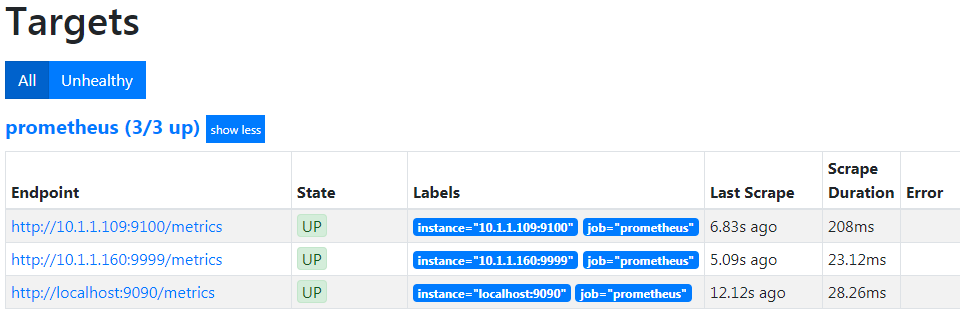
sudo systemctl restart prometheus

Now if we return to our Prometheus GUI (http://10.1.1.110:9090/targets) to check which targets we are scraping we can see three targets, including our new node at 10.1.1.160.

Creating a new graph in Grafana

Righto…

We now have our custom exporter reading our values successfully, let’s visualize the results in Grafana!

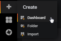
From the Grafana home page select the Add icon (it’s a ‘+’ sign) from the left hand menu bar and from there select dashboard. Technically this is adding a dashboard, but at this stage we’re just going to implement a single graph.

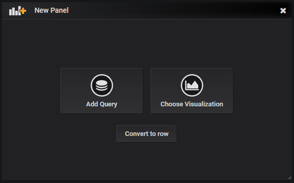
The next screen will allow us to start the process by either choosing the type of visualisation (Line graph, gauge, table, list etc) or by simply adding a query. In our case we’re going to take a simple route and select ‘Add Query’. Grafana will use the default visualisation which is the line graph.

Now we are presented with our graph with no data assigned.

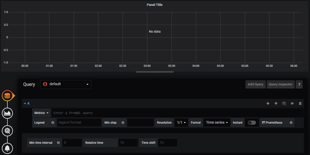
By adding a query, we are selecting the data source that will be used to populate the graph. The main source that our Query will be selecting against is already set as the default Prometheus. All that remains for us is to select which metric we want from Prometheus.

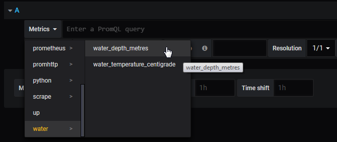
We do that by clicking on the ‘Metrics’ drop down which will provide a range of different potential sources. Scroll down the list and we will see ‘water’ which is the first part of our metric name (the domain) that we assigned. Click on that and we can see the two metrics that we set up to record. Select ‘water_depth_metres’.

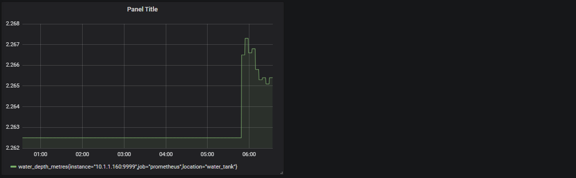
That will instantly add the metric data stream with whatever data has been recorded up to that point. Depending on how fast you are, that could be only a few data points or, as you can see from the graph below, there could be a bit more.

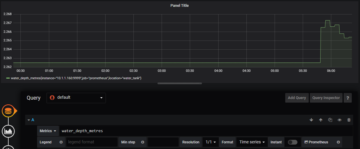
Spectacularly we have our graph of water depth!

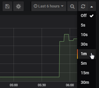
At the moment it’s a static graph, so let’s change it to refresh every minute by selecting the drop-down by the refresh symbol in the top right corner and selecting ‘1m’.

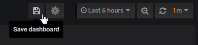
Now all we have remaining is to save our masterpiece so that we can load it again as desired. To do this, go to the save icon at the top of the screen and click it.

The following dialogue will allow us to give our graph a fancy name and then we slick on the ‘Save’ button.

There it is! It looks slightly unusual stuck on the left hand side of the screen, but that’s because it is a single graph (or panel) in a row that is built for two. As an exercise for the reader, go through the process of adding a second panel by selecting the ‘Add Panel’ icon on the top of the screen.

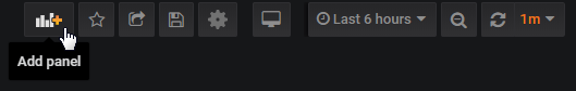
This time select the water temperature as the metric. You might want to move the panel about to get it in the righ place and you can adjust the size of the panels by grabbing the corners of the individual panels. Ultimately something like the following is the result!

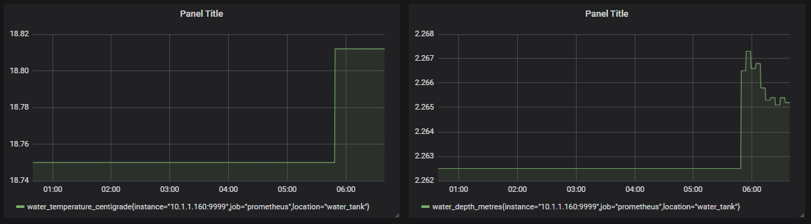
Not bad for a few mouse clicks. Make sure that you save the changes and you’re done!