An Embedded Probabilistic Programming Language
A probabilistic program describes a generative model in ordinary code: it draws latent parameters from priors, then ties those parameters to observed data through likelihoods. A probabilistic programming language (PPL) separates the model from the inference. You write the model once; the language supplies a generic engine that returns the posterior distribution of the parameters given the data. The same model can be fit by several different engines without rewriting a line.
This chapter builds a small but complete PPL in Common Lisp. It provides a macro DSL for declaring models and three inference engines written from scratch: random-walk Metropolis-Hastings, Hamiltonian Monte Carlo with automatic differentiation, and mean-field variational inference. A terminal REPL and text plots let you inspect the results.
The example program for this chapter is in the file 11_probabilistic_dsl.lisp.
What Inference Computes
Chapter 9 introduced Bayesian updating for a single conjugate pair, where the posterior fell out as a closed-form Beta. Real models rarely have that luxury. A probabilistic program encodes the joint distribution 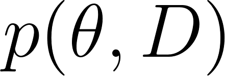 over latent parameters
  and data
  . The program draws each latent from a prior with
 sample and ties latents to data through a likelihood with observe. Inference targets the posterior
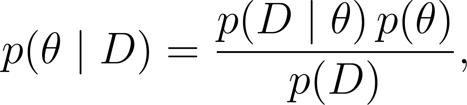
where the marginal likelihood 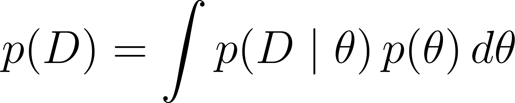 is usually an intractable integral over the parameter space.
The key observation that makes all three engines in this chapter work is that we never need 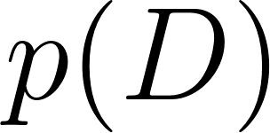 . Every acceptance ratio and every gradient involves a ratio or a difference of log densities, and the constant
 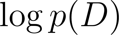 cancels. So each engine needs only the unnormalized log posterior

The program computes 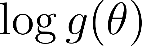 for any . The engine’s job is to explore the shape of
  and report where its mass sits. Sampling engines return a set of draws whose empirical distribution approximates the posterior; the variational engine returns a simple approximating distribution tuned to match it.
Unconstrained Space and the Jacobian
A prior often lives on a bounded set. A standard deviation is positive; a probability lies in 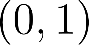 . The samplers in this chapter move on the whole real line, so each latent is reparameterized. We work in an unconstrained space
 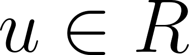 and map back to the natural scale with a transform
 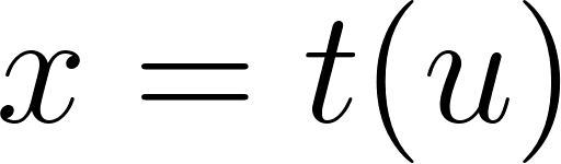 :
: 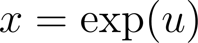 for positive support,
  for the unit interval, and a scaled sigmoid for a bounded interval.
A change of variables bends the density. For the transformed variable the density picks up the Jacobian:

For the Jacobian term is  . For the sigmoid it is
  . The DSL applies these corrections automatically, so the model author never writes a transform or a Jacobian by hand. This keeps the model readable and keeps the math correct.
Three Ways to Find the Posterior
There are three standard computational routes from 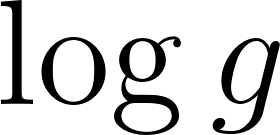 to the posterior, and this chapter implements all three.
Metropolis-Hastings (MCMC). Start at a point  . Propose a new point
  . Accept it with probability

If accepted, the chain moves to 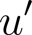 ; otherwise it stays. Under mild conditions the chain’s stationary distribution is the posterior. The method is simple and needs no gradients, but it mixes slowly in high dimensions because random proposals wander.
Hamiltonian Monte Carlo. Treat 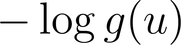 as a potential energy and add a momentum variable
  with kinetic energy
 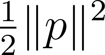 . The total energy is

Simulate the Hamiltonian dynamics with the leapfrog integrator for several steps, which slides the state along the posterior’s level sets. Accept the endpoint with probability  . Long, low-rejection moves need the gradient of , which we get exactly from automatic differentiation rather than finite differences. HMC mixes far better than random-walk Metropolis in moderate dimensions.
Variational inference. Instead of simulating the posterior, fit a simple distribution 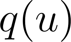 to it. We use a factorized Normal
 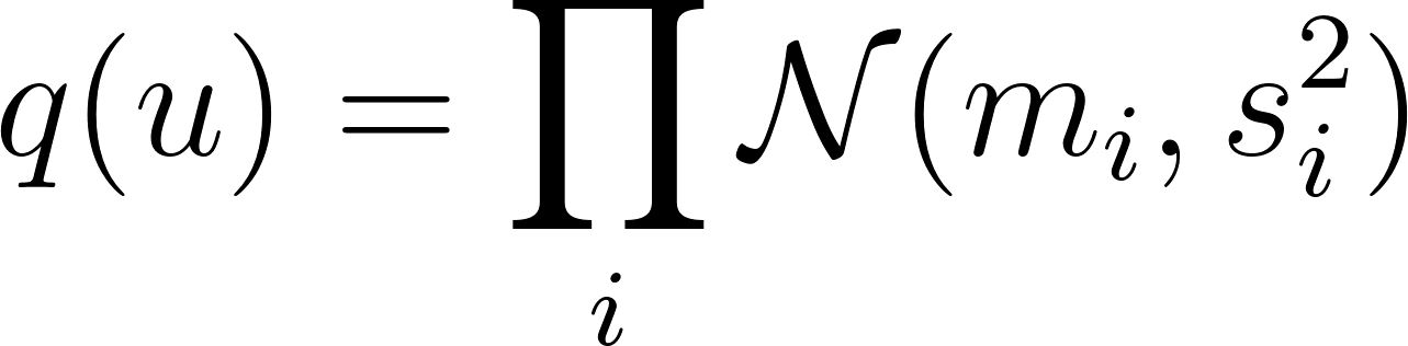 . Fitting
  means maximizing the Evidence Lower Bound

where 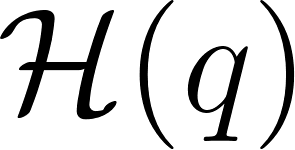 is the entropy of . The reparameterization trick writes a sample as
  with
with 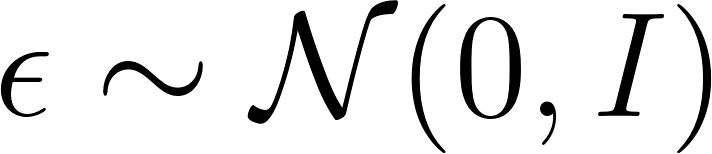 , so the expectation becomes a differentiable function of
 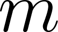 and
and  . The same automatic differentiation supplies the gradient, and Adam ascends the ELBO. Variational inference is fast and deterministic, but it approximates the posterior with a shape (independent Gaussians) that may not match the truth.
The next sections show how the file builds the pieces these engines share: automatic differentiation, a distribution library, support transforms, and the model DSL.
Forward-Mode Automatic Differentiation
HMC and variational inference both need the gradient of . The file implements forward-mode automatic differentiation with dual numbers. A dual number carries a value together with the full gradient vector of that value with respect to the model parameters. Every primitive operation propagates the gradient by the chain rule, so a single evaluation of the log density yields both its value and its exact gradient.

For a unary function 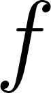 with derivative
 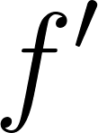 , the rule is
  . For a binary function the partials combine by the chain rule. Constants stay plain doubles, so Metropolis-Hastings, which needs no gradient, pays no AD overhead.
 1 (defstruct (dual (:constructor make-dual (v g)))
 2   (v 0.0d0 :type double-float)   ; the value
 3   (g))                            ; simple-vector of partials, length *ad-dim*
 4
 5 (defun d-unary (x val dval)
 6   "Build f(x): VAL is f(value), DVAL is f'(value). Returns a dual iff X is."
 7   (if (dual-p x)
 8       (let* ((n *ad-dim*) (gx (dual-g x))
 9              (g (make-array n :element-type 'double-float)))
10         (dotimes (i n) (setf (aref g i) (* dval (aref gx i))))
11         (make-dual val g))
12       val))
13
14 (defun d-binary (a b val da db)
15   "Build f(a,b): VAL is the value, DA and DB the partials wrt a and b."
16   (if (or (dual-p a) (dual-p b))
17       (let* ((n *ad-dim*) (ga (dg a)) (gb (dg b))
18              (g (make-array n :element-type 'double-float)))
19         (dotimes (i n)
20           (setf (aref g i) (+ (* da (aref ga i)) (* db (aref gb i)))))
21         (make-dual val g))
22       val))
On top of these two combinators, the file defines differentiable versions of the arithmetic operators. Each one passes the right partials through d-binary or d-unary:
1 (defun g+ (a b) (d-binary a b (+ (dv a) (dv b)) 1.0d0 1.0d0))
2 (defun g* (a b) (let ((av (dv a)) (bv (dv b)))
3                   (d-binary a b (* av bv) bv av)))
4 (defun gexp (x)
5   ;; Cap the exponent to keep exp from overflowing to infinity.
6   (let* ((ax (min 700.0d0 (dv x))) (e (exp ax))) (d-unary x e e)))
7 (defun glog (x)
8   ;; Clamp the argument into the positive domain of log.
9   (let ((ax (max 1d-300 (dv x)))) (d-unary x (log ax) (/ 1.0d0 ax))))
The entry point seeds coordinate 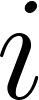 with the unit dual
  (value
  everywhere except partial set to
  ), runs the function once, and reads the value and full gradient off the result. One pass gives the whole gradient vector:
 1 (defun ad-gradient (f x)
 2   "Differentiate scalar F at point X (a vector of doubles).
 3    Seeds coordinate i with the unit dual e_i, runs F once, and reads the
 4    value and full gradient off the result. Returns (values value gradient)."
 5   (let* ((n (length x))
 6          (*ad-dim* n)
 7          (duals (make-array n)))
 8     (dotimes (i n)
 9       (let ((g (make-array n :element-type 'double-float :initial-element 0.0d0)))
10         (setf (aref g i) 1.0d0)
11         (setf (aref duals i) (make-dual (coerce (aref x i) 'double-float) g))))
12     (let ((r (funcall f duals)))
13       (values (dv r) (dg r)))))
The cost is one evaluation of per parameter dimension, which is fine for the small models in this chapter. (Reverse-mode AD would be cheaper for functions with many inputs and one output, but forward mode is simple to build and exact.) The numerical guards in 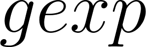 and
and  matter: a divergent HMC trajectory can push a parameter to an extreme value, and clamping keeps the gradient finite so the trajectory can be rejected rather than crashing the sampler.
The Distribution Library
Each distribution is a small record holding three things: a log-density function written with the differentiable operators, a plain sampler used to initialize chains, and the support of the distribution (:real, :positive, :unit, :bounded, or :discrete). The support fixes the transform to unconstrained space.
 1 (defstruct (dist (:conc-name dist-))
 2   name logpdf sampler (support :real) (lo nil) (hi nil))
 3
 4 (defun normal (mu sigma)
 5   "Normal(mu, sigma) on the whole real line."
 6   (make-dist
 7    :name 'normal :support :real
 8    :sampler (lambda () (rnorm (dv mu) (dv sigma)))
 9    :logpdf (lambda (x)
10              (let ((z (g/ (g- x mu) sigma)))
11                (g- (g- (gneg (g* 0.5d0 (gsquare z))) (glog sigma))
12                    (* 0.5d0 +log2pi+))))))
The log-density is built from g-, g*, g/, gsquare, and glog, so it carries gradients when its inputs are duals and computes plainly when they are doubles. The parameters  and
and 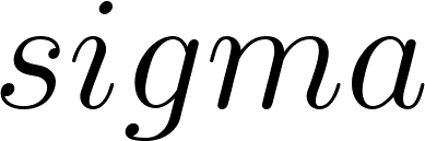 may themselves be duals, which is what makes hierarchical models work: a likelihood mean can depend on other latents, and the gradient still flows through.
The library supplies Normal, Half-Normal, Exponential, Gamma, Beta, Uniform, Bernoulli, and Poisson. The Beta and Gamma log densities use a Lanczos approximation to  , and the Poisson likelihood uses
  . These are the same special functions that appeared in Chapter 5 (continuous distributions) and Chapter 9 (the Beta-Bernoulli update), restated here so the file stands alone.
Support Transforms
Two small functions handle the mapping between constrained and unconstrained space. constrain-support maps an unconstrained real back to the distribution’s support, and  returns the log Jacobian of that map. Both are written with the differentiable operators so the Jacobian term enters the gradient correctly.
 1 (defun constrain-support (support lo hi u)
 2   "Map an unconstrained real U to the distribution's support."
 3   (case support
 4     (:real u)
 5     (:positive (gexp u))
 6     (:unit (sigmoidg u))
 7     (:bounded (g+ lo (g* (- hi lo) (sigmoidg u))))
 8     (t u)))
 9
10 (defun log-jac-support (support lo hi u)
11   "Log absolute Jacobian log|dx/du| of the support transform at U."
12   (case support
13     (:real 0.0d0)
14     (:positive u)                               ; d/du exp(u) = exp(u); log = u
15     (:unit (let ((s (sigmoidg u)))
16              (g+ (glog s) (glog (g- 1.0d0 s)))))
17     (:bounded (let ((s (sigmoidg u)))
18                 (g+ (log (- hi lo)) (g+ (glog s) (glog (g- 1.0d0 s))))))
19     (t 0.0d0)))
For 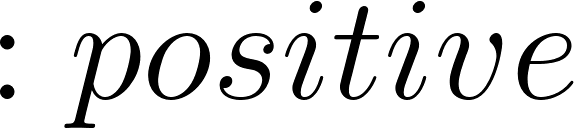 support the Jacobian term is just , because
  and
and  . For
. For 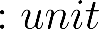 support it is
  , the log of the sigmoid derivative. The sampler side uses a plain
  and
and 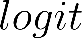 to invert the transform when placing initial values.
The Model DSL: defmodel, sample, observe
The macro defmodel defines a function that, when called with data, returns a model object. The model body runs under a dynamic context in one of two modes:
:initdiscovers the latents in order and picks dispersed starting values.:densityreads a parameter vector and accumulates the unconstrained log posterior (prior plus Jacobian plus likelihood).
The body never mentions transforms or gradients. sample and observe handle all of it.
1 (defmacro defmodel (name (&rest params) &body body)
2   "Define a probabilistic model NAME with formal data PARAMS. Inside BODY use
3    (sample name dist) to declare a latent and (observe dist datum) to score
4    data. Calling (NAME data...) returns a model object to hand to `infer`."
5   `(defun ,name ,params
6      (make-model :name ',name :param-names ',params
7                  :thunk (lambda () ,@body))))
sample declares a latent. In 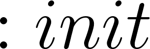 mode it records the latent’s support and returns a starting value. In
 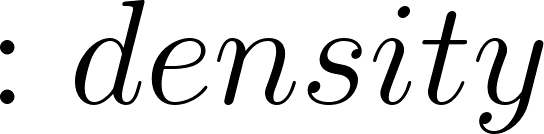 mode it reads the next parameter from the vector, transforms it to the natural scale, and adds the prior log density plus the Jacobian to the running total:
 1 (defun sample (name dist)
 2   "Declare a latent variable NAME with prior DIST; return its current value."
 3   (let ((ctx *ctx*))
 4     (ecase (ctx-mode ctx)
 5       (:init
 6        ;; Start each chain dispersed but sane: uniform in [-2,2] on the
 7        ;; unconstrained line. This over-disperses relative to typical
 8        ;; posteriors (good for R-hat) without the extreme values a vague
 9        ;; prior draw could produce.
10        (let* ((u0 (- (* 4.0d0 (runif)) 2.0d0))
11               (x0 (constrain-support (dist-support dist)
12                                      (dist-lo dist) (dist-hi dist) u0)))
13          (push (make-pstate :name name :support (dist-support dist)
14                             :lo (dist-lo dist) :hi (dist-hi dist))
15                (ctx-supports ctx))
16          (push u0 (ctx-inits ctx))
17          x0))
18       (:density
19        (let* ((i (ctx-index ctx))
20               (u (aref (ctx-params ctx) i))
21               (x (constrain-support (dist-support dist)
22                                     (dist-lo dist) (dist-hi dist) u)))
23          (setf (ctx-index ctx) (1+ i))
24          (setf (ctx-logdens ctx)
25                (g+ (ctx-logdens ctx)
26                    (g+ (funcall (dist-logpdf dist) x)
27                        (log-jac-support (dist-support dist)
28                                         (dist-lo dist) (dist-hi dist) u))))
29          x)))))
30
31 (defun observe (dist value)
32   "Score an observed VALUE under likelihood DIST. Ignored while initializing."
33   (let ((ctx *ctx*))
34     (when (and ctx (eq (ctx-mode ctx) :density))
35       (setf (ctx-logdens ctx)
36             (g+ (ctx-logdens ctx)
37                 (funcall (dist-logpdf dist) (coerce value 'double-float)))))
38     value))
The same body serves both modes because sample and observe dispatch on ctx-mode. Running the body once in mode builds the latent list and the start vector; running it in mode with a parameter vector builds the log posterior. Two thin wrappers package these:
 1 (defun model-init (model)
 2   "Run MODEL once in init mode. Returns (values init-u-vector pstates)."
 3   (let ((*ctx* (make-ctx :mode :init)))
 4     (funcall (model-thunk model))
 5     (values (coerce (nreverse (ctx-inits *ctx*)) 'vector)
 6             (nreverse (ctx-supports *ctx*)))))
 7
 8 (defun model-logdensity (model)
 9   "Return a closure u-vector -> unconstrained log posterior (dual-aware)."
10   (lambda (u)
11     (let ((*ctx* (make-ctx :mode :density :params u)))
12       (funcall (model-thunk model))
13       (ctx-logdens *ctx*))))
The dynamic variable 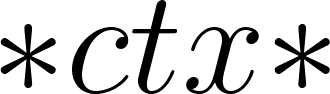 carries the mode and the accumulator, so the model body reads like a direct description of the generative process. This is the whole point of an embedded DSL: the model is just a Lisp function, and the host language’s machinery does the rest.
The Example Data
The file ships three data generators, one per built-in model. Before fitting, it helps to see what the data look like.
 1 (defun example-coin-data ()
 2   "40 flips with 28 heads (true bias near 0.7)."
 3   (append (make-list 28 :initial-element 1) (make-list 12 :initial-element 0)))
 4
 5 (defun example-normal-data (&optional (n 60))
 6   "N draws from Normal(5, 2)."
 7   (let ((v (make-dvec n)))
 8     (dotimes (i n v) (setf (aref v i) (rnorm 5.0d0 2.0d0)))))
 9
10 (defun example-regression-data (&optional (n 40))
11   "N points from y = 1 + 2x + Normal(0,1). Returns (values xs ys)."
12   (let ((xs (make-dvec n)) (ys (make-dvec n)))
13     (dotimes (i n (values xs ys))
14       (let ((x (- (* 4.0d0 (runif)) 2.0d0)))
15         (setf (aref xs i) x
16               (aref ys i) (+ 1.0d0 (* 2.0d0 x) (rnorm 0.0d0 1.0d0)))))))
The three formats are:
- Coin: a list of and , here
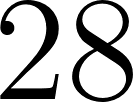 ones and
 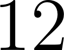 zeros:
 (1 1 1 0 1 ... 1 0 0). - Normal: a vector of doubles drawn from
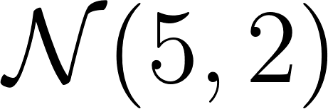 , for example
 #(4.83 6.21 3.40 5.57 ...). - Regression: two parallel vectors
 and
and 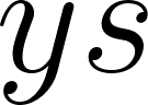 , where each
  with
with 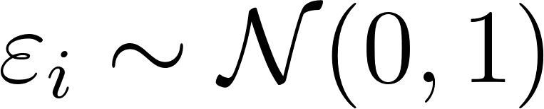 .
.
Because the global random state is freshly seeded on every load, the exact data (and so the exact posterior) differ slightly each session. The true parameters stay fixed: coin bias near 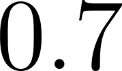 , normal mean
  and standard deviation
  , regression intercept , slope , noise .
The Three Inference Engines
Metropolis-Hastings
The simplest engine is a random-walk Metropolis sampler in unconstrained space. At each iteration it adds isotropic Gaussian noise to the current point, evaluates at the proposal, and accepts with the Metropolis ratio. Divergent proposals (infinite or NaN log density) are rejected. The engine records the acceptance rate and returns posterior draws transformed back to the natural scale.
 1 (defun engine-mh (model &rest args)
 2   "Random-walk Metropolis in unconstrained space. Gradient-free MCMC."
 3   (let* ((iters (getf args :iters 6000))
 4          (burn  (getf args :burn 2000))
 5          (step  (getf args :step 0.4d0))
 6          (thin  (getf args :thin 1)))
 7     (multiple-value-bind (u0 pstates) (model-init model)
 8       (let* ((f (model-logdensity model))
 9              (dim (length u0))
10              (u (to-dvec u0))
11              (lp (dv (funcall f u)))
12              (rows nil) (nacc 0) (nprop 0))
13         (dotimes (it iters)
14           (let ((prop (make-dvec dim)))
15             (dotimes (i dim)
16               (setf (aref prop i) (+ (aref u i) (rnorm 0.0d0 step))))
17             (let ((lp2 (dv (funcall f prop))))
18               (incf nprop)
19               (when (and (finitep lp2)
20                          (< (log (max 1d-300 (runif))) (- lp2 lp)))
21                 (setf u prop lp lp2) (incf nacc))))
22           (when (and (>= it burn) (zerop (mod (- it burn) thin)))
23             (push (constrain-draw pstates u) rows)))
24         (values (nreverse rows) pstates
25                 (list :accept-rate (/ nacc (max 1 nprop) 1.0d0)))))))
The proposal scale 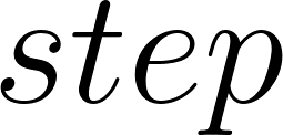 controls the tradeoff between acceptance rate and move size. Too small and nearly every proposal is accepted but the chain crawls; too large and nearly every proposal is rejected and the chain stalls. A rate around
  to
to  usually mixes well for random-walk Metropolis.
Hamiltonian Monte Carlo
HMC treats as a potential energy. Each iteration draws a fresh momentum 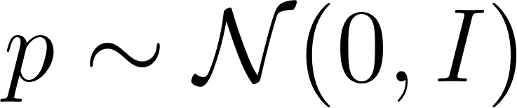 , then simulates the Hamiltonian dynamics with the leapfrog integrator. The integrator alternates half-step momentum updates with full-step position updates, using the gradient of the potential at each step. The gradient comes from
 ad-gradient, so it is exact.
 1 (labels ((potential-grad (uv)
 2            ;; Potential U = -log g; its gradient is -grad(log g).
 3            (multiple-value-bind (val g) (ad-gradient f uv)
 4              (let ((ng (make-dvec dim)))
 5                (dotimes (i dim) (setf (aref ng i) (- (aref g i))))
 6                (values (- val) ng)))))
 7   (let ((steps (1+ (random steps0)))      ; jitter path length to avoid resonance
 8         (p (randn-vec dim))
 9         (cur-pos (copy-seq u)))
10     (multiple-value-bind (cur-pot cur-grad) (potential-grad cur-pos)
11       (when (finitep cur-pot)
12         (let ((cur-kin 0.0d0))
13           (dotimes (i dim) (incf cur-kin (* 0.5d0 (aref p i) (aref p i))))
14           (let ((pp (copy-seq p)) (uu (copy-seq cur-pos))
15                 (grad cur-grad) (prop-pot cur-pot))
16             (dotimes (i dim)           ; half step for momentum
17               (decf (aref pp i) (* 0.5d0 eps (aref grad i))))
18             (block leapfrog
19               (dotimes (l steps)       ; full leapfrog steps
20                 (dotimes (i dim) (incf (aref uu i) (* eps (aref pp i))))
21                 (multiple-value-bind (vv gg) (potential-grad uu)
22                   (setf prop-pot vv grad gg)
23                   (unless (finitep vv) (return-from leapfrog)) ; diverged
24                   (when (< l (1- steps))
25                     (dotimes (i dim)
26                       (decf (aref pp i) (* eps (aref grad i))))))))
27             (dotimes (i dim)           ; final half step
28               (decf (aref pp i) (* 0.5d0 eps (aref grad i))))
29             (let ((prop-kin 0.0d0))
30               (dotimes (i dim)
31                 (incf prop-kin (* 0.5d0 (aref pp i) (aref pp i))))
32               (incf nprop)
33               (let ((alpha (if (and (finitep prop-pot) (finitep prop-kin))
34                                (min 1.0d0 (exp (- (+ cur-pot cur-kin)
35                                                   (+ prop-pot prop-kin))))
36                                0.0d0)))
37                 (when (< (runif) alpha) (setf u uu) (incf nacc))))))))))
Two details matter in practice. The path length is jittered each iteration (steps = 1 + random(steps0)) so the integrator cannot resonate with the target’s curvature, which would cripple mixing. And a divergent trajectory (the potential becomes infinite) breaks out of the leapfrog loop early and is rejected, the same safety net as in Metropolis. During warmup a Nesterov dual-averaging scheme adapts the step size 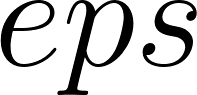 toward a target acceptance rate of
  , then freezes it to the running average for the sampling phase. This is the adaptation recipe from Hoffman and Gelman’s NUTS paper, applied to plain HMC.
Variational Inference
The variational engine fits a factorized Normal by maximizing the ELBO. It stores the mean and the log standard deviation 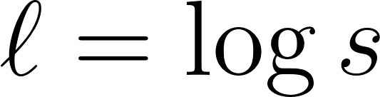 (so the standard deviation stays positive for free). Each iteration draws
  samples from , and for each sample it computes the gradient of at . The reparameterization trick moves the gradient of the expectation onto and
  :
:

The 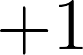 on the log-standard-deviation gradient is the entropy term : it widens unless the data pulls the mean toward higher . Adam ascends both parameter sets.
 1 (dotimes (s mc)
 2   (let ((eps (randn-vec dim)) (u (make-dvec dim)))
 3     (dotimes (i dim)
 4       (setf (aref u i) (+ (aref m i)
 5                           (* (exp (aref ls i)) (aref eps i))))) ; u = m + s*eps
 6     (multiple-value-bind (val g) (ad-gradient f u)
 7       (when (and (finitep val) (every #'finitep g))
 8         (dotimes (i dim)
 9           ;; dELBO/dm = grad ; dELBO/dls = grad*sd*eps + 1 (entropy).
10           (incf (aref gm i) (aref g i))
11           (incf (aref gl i)
12                 (+ (* (aref g i) (exp (aref ls i)) (aref eps i))
13                    1.0d0)))))))
After Adam converges, the engine draws a large sample from the fitted and returns those draws, transformed back to the natural scale, as its posterior summary. Variational inference is fast and deterministic, but its answer is only as good as the factorized Normal approximation. For a unimodal posterior on the unconstrained scale it does well; for a posterior with strong correlations or multiple modes it can miss.
Diagnostics: ESS and R-hat
Sampling only approximates the posterior, so the file reports two standard diagnostics alongside each fit.
The effective sample size (ESS) measures how many independent draws the autocorrelated chain is worth. If consecutive draws are correlated, the chain carries less information than its length suggests. Geyer’s initial positive sequence estimator sums the autocorrelations until they turn negative:
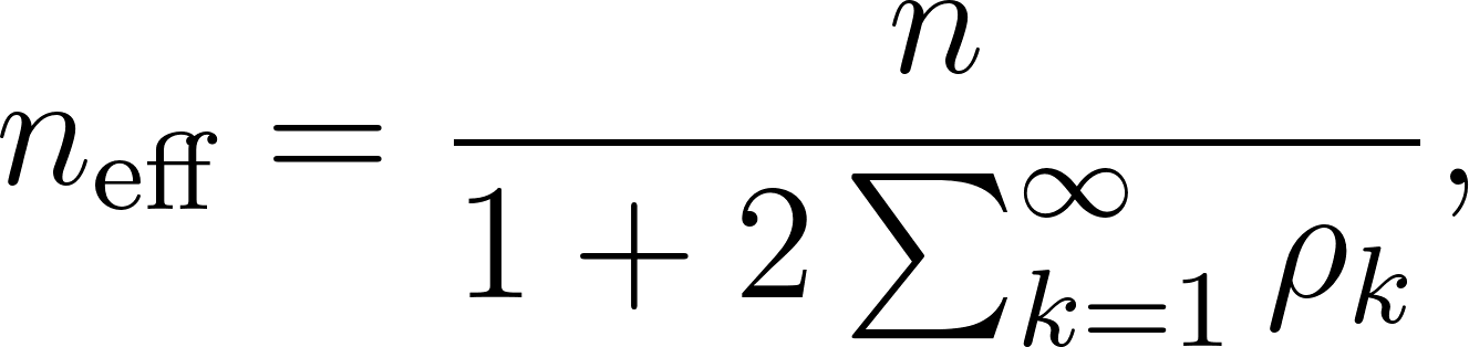
where 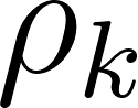 is the lag-
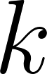 autocorrelation. An ESS near
  means the draws are nearly independent; an ESS far below means the chain mixes poorly and you should run longer or switch engines.
 1 (defun ess (series)
 2   "Effective sample size from Geyer's initial positive autocorrelation sum."
 3   (let* ((n (length series)) (m (mean-of series))
 4          (var (/ (reduce #'+ (map 'list (lambda (x) (expt (- x m) 2)) series))
 5                  n)))
 6     (if (<= var 0.0d0)
 7         (coerce n 'double-float)
 8         (let ((s 0.0d0))
 9           (loop for lag from 1 below n
10                 for rho = (autocorr series m var lag)
11                 while (> rho 0.0d0)
12                 do (incf s rho))
13           (clampd (/ n (+ 1.0d0 (* 2.0d0 s))) 1.0d0 (coerce n 'double-float))))))
The Gelman-Rubin 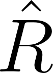 (R-hat) compares the variance within each chain to the variance between chains. Run several chains from dispersed starts. If they all sample the same posterior, the between-chain variance should match the within-chain variance and
 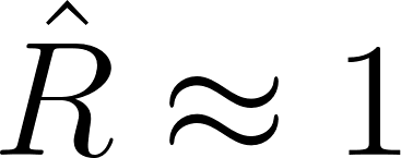 . If the chains disagree, rises above , signalling that the chains have not converged. The statistic is

with  the between-chain variance and
  the average within-chain variance. A common rule of thumb is to trust the fit when
 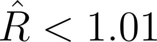 for every parameter. R-hat needs at least two chains; with one chain the file reports ESS only.
Running the Example
Load the file and it drops you into the PPL REPL:
1 rlwrap sbcl --load 11_probabilistic_dsl.lisp
Type demo at the ppl> prompt for a guided tour, or fit a model directly. The (demo) function fits the coin and the Normal models, plots their posteriors, and compares all three engines against the exact Beta answer. Because the random state is freshly seeded each session, your numbers will differ slightly from those below, but the patterns hold.
The Coin Bias
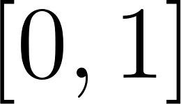
The coin model puts a 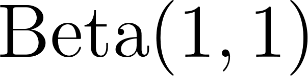 prior (uniform on
  ) on the bias and scores
  flips, of them heads, with a Bernoulli likelihood:
1 (defmodel coin-model (flips)
2   "Coin bias: p ~ Beta(1,1), each flip ~ Bernoulli(p)."
3   (let ((p (sample :p (beta-dist 1.0d0 1.0d0))))
4     (dolist (f flips) (observe (bernoulli p) f))))
With a prior and heads, tails, the exact posterior is 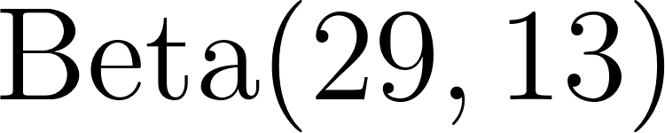 with mean
  (Chapter 9’s conjugate update). HMC with two chains reproduces it:
 1 Posterior summary  [method hmc, 2000 draws, 2 chain(s)]
 2   param    mean       sd         2.5%       50%        97.5%      ess      R-hat
 3   p            0.6859     0.0713     0.5321     0.6890     0.8241    2000.   1.000
 4   acceptance rate: 0.853
 5
 6 posterior of p
 7       0.484 | ###
 8       0.506 | ####
 9       0.527 | ###
10       0.549 | ######
11       0.570 | #########
12       0.592 | #################
13       0.613 | ##########################
14       0.635 | ####################################
15       0.656 | ####################################
16       0.678 | #######################################
17       0.699 | ############################################
18       0.721 | ########################################
19       0.742 | #################################
20       0.764 | ############################
21       0.785 | #################
22       0.807 | ########
23       0.828 | ######
24       0.850 | ####
25       0.871 | #
The posterior mean  sits next to the exact
  . The 95% credible interval
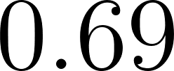
  is what the conjugate gives. The histogram is the shape of that Beta density: roughly symmetric, peaked near
  , tapering to both sides. ESS equals the full
  draws and R-hat is
  , so the two chains agree and mix almost perfectly. The acceptance rate
 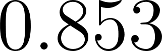 is right at the HMC target of .
Three Engines Versus the Exact Answer
The demo fits the same coin with each engine and checks the posterior mean against the exact 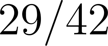 :
:
1   engine         E[p]       abs err
2   Metropolis         0.6896     0.0009
3   HMC                0.6884     0.0021
4   Variational        0.6746     0.0159
All three land within a couple of percentage points of . Metropolis and HMC, both sampling the posterior directly, are essentially exact up to Monte Carlo noise. Variational inference is less accurate here because the factorized Normal is fit in unconstrained space and then pushed through the sigmoid; the mean of a transformed Normal is not the transform of the mean, so the bias shifts slightly. This is the usual cost of variational inference: speed and determinism in exchange for a small, controllable bias.
Unknown Mean and Spread
The mean-var model puts a 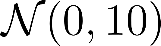 prior on the mean, a Half-Normal
 prior on the standard deviation, and scores
 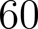 draws from with a Normal likelihood:
1 (defmodel mean-var-model (data)
2   "Unknown mean and spread: mu ~ Normal(0,10), sigma ~ HalfNormal(5),
3    each datum ~ Normal(mu, sigma)."
4   (let ((mu (sample :mu (normal 0.0d0 10.0d0)))
5         (sigma (sample :sigma (half-normal 5.0d0))))
6     (loop for x across data do (observe (normal mu sigma) x))))
Two chains recover both parameters:
1 Posterior summary  [method hmc, 2400 draws, 2 chain(s)]
2   param    mean       sd         2.5%       50%        97.5%      ess      R-hat
3   mu           5.0625     0.3098     4.4528     5.0655     5.6644    1768.   1.000
4   sigma        2.4944     0.2326     2.0893     2.4749     3.0082    1566.   1.000
5   acceptance rate: 0.846
The posterior mean of is 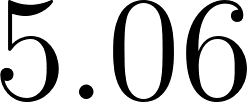 , bracketing the true . The posterior mean of is
 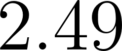 : with only draws the sample standard deviation has upward scatter, and the half-normal prior adds a gentle pull, so the estimate sits a little above the true . The credible intervals cover both true values. R-hat is for both and ESS is high, so the chains agree and mix well.
Bayesian Linear Regression
The regression model puts Normal priors on the intercept and slope and a Half-Normal prior on the noise, then scores 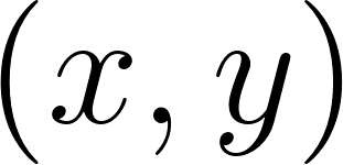 points. The mean
 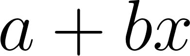 is built with the differentiable operators
 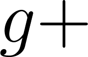 and
and 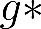 , so HMC and VI get gradients through it:
1 (defmodel regression-model (xs ys)
2   "Linear regression y ~ Normal(a + b x, sigma). The mean a + b*x is built
3    with the differentiable ops so HMC and VI get gradients through it."
4   (let ((a (sample :a (normal 0.0d0 10.0d0)))
5         (b (sample :b (normal 0.0d0 10.0d0)))
6         (sigma (sample :sigma (half-normal 5.0d0))))
7     (loop for x across xs for y across ys
8           do (observe (normal (g+ a (g* b x)) sigma) y))))
Two chains recover the true line  with noise :
1 Posterior summary  [method hmc, 2400 draws, 2 chain(s)]
2   param    mean       sd         2.5%       50%        97.5%      ess      R-hat
3   a            1.0078     0.1612     0.6836     1.0036     1.3277    1813.   1.000
4   b            1.9109     0.1508     1.6102     1.9089     2.2197    2005.   1.000
5   sigma        1.0118     0.1236     0.8070     0.9959     1.2813    1283.   1.001
6   acceptance rate: 0.837
The intercept  and slope
 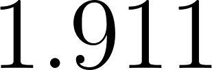 both cover their true values of and , and the noise
  covers the true . This is the first model with a linear predictor: the likelihood mean depends on two latents at once. The AD pass threads the gradient through and without the model author doing anything special, which is what makes the DSL usable for models more complex than a single prior.
Reading the Diagnostics
The same coin fit by random-walk Metropolis shows why diagnostics matter. A standalone run gives:
1 Posterior summary  [method mh, 10000 draws, 2 chain(s)]
2   param    mean       sd         2.5%       50%        97.5%      ess      R-hat
3   p            0.6903     0.0694     0.5465     0.6930     0.8153    2234.   1.000
4   acceptance rate: 0.533
The posterior mean is right on the exact , but note the cost. Metropolis used  iterations to get ESS
 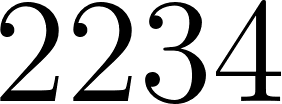 , while HMC got ESS from only draws. Each Metropolis draw is worth roughly a fifth of an independent draw; each HMC draw is worth nearly one. The autocorrelation plot makes the cause visible:
 1 autocorrelation of p
 2   lag   0  1.000 |########################################
 3   lag   1  0.654 |##########################
 4   lag   2  0.431 |#################
 5   lag   3  0.294 |############
 6   lag   4  0.211 |########
 7   lag   5  0.149 |######
 8   lag   6  0.110 |####
 9   lag   7  0.080 |###
10   lag   8  0.060 |##
11   lag   9  0.041 |##
12   lag  10  0.022 |#
13   lag  11  0.017 |#
14   lag  12  0.017 |#
15   lag  13  0.018 |#
16   lag  14  0.006 |
17   lag  15 -0.008 |
The autocorrelation decays slowly: even at lag  it is still positive. The area under this curve is the
 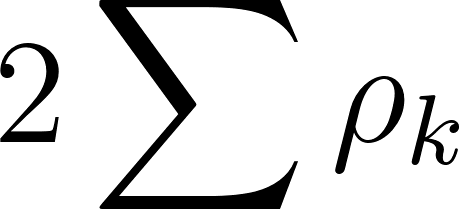 in the ESS denominator, and that area is large, so ESS is far below . HMC’s leapfrog moves slide along the posterior and decorrelate quickly, which is why its autocorrelation drops to near zero within a few lags and its ESS sits near . R-hat is for both engines, so both have converged; the difference is purely efficiency. This is the practical case for HMC over random-walk Metropolis in even modest dimensions.
Wrap Up
This chapter assembled a working probabilistic programming language from three ingredients: a tiny DSL (defmodel, sample, observe) that lets you state a model as plain Lisp; a layer of forward-mode automatic differentiation that turns a log-density function into its gradient; and three inference engines that share the same model and the same unnormalized log posterior. Metropolis-Hastings is the simple, gradient-free baseline. HMC adds a gradient and a momentum and mixes far better. Variational inference trades exact sampling for a fast, deterministic approximation.
The whole system fits in one file of roughly  lines and uses only Common Lisp primitives plus a few SBCL-specific float-trap masks. It connects the earlier chapters into a single tool: the Normal, Beta, Gamma, and Poisson distributions from Chapters 5 and 9, the Monte Carlo idea from Chapter 8, and the Markov chain theory from Chapter 10 all reappear here. The Metropolis-Hastings chain is a Markov chain whose stationary distribution is the posterior, and the convergence diagnostics R-hat and ESS measure exactly the mixing behavior Chapter 10 analyzed.
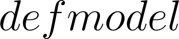
The DSL is extensible. Adding a new distribution means writing one  call with a log density and a sampler. Adding a new model means writing one
  form. To go further you might add a Student-t likelihood for robust regression, a log-normal prior, a No-U-Turn Sampler to tune HMC’s path length automatically, or a reparameterization that handles posteriors with strong correlations. The framework is already there; the model and the engine are finally separate.
Problem Set
Problem 11.1. For the coin model with a prior and heads in flips, the exact posterior is with mean and variance  . Compute the exact posterior standard deviation and compare it with the
 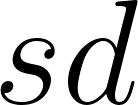 column the HMC summary reports (about
 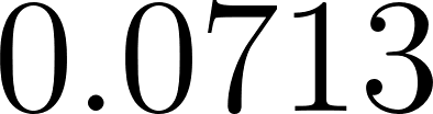 ).
).
Problem 11.2 (Two modes). Trace through the coin model body in both and modes. In mode, what value does sample return, and what gets pushed onto the context? In mode with parameter vector 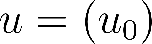 , write down the three terms that
 sample adds to ctx-logdens (the Beta prior log density, the Jacobian, and the Bernoulli likelihood is added later by observe). Why does observe do nothing in mode?
Problem 11.3 (ESS and efficiency). The Metropolis run used iterations to reach ESS , while HMC used draws to reach ESS . How many Metropolis iterations would you need to match HMC’s effective draws, assuming the same efficiency? What does this say about the per-draw cost of random-walk Metropolis versus HMC?
Problem 11.4 (R-hat). Run the coin model with  and read the R-hat column. Now deliberately break mixing by setting the HMC step size very large (
:step 2.0d0) with few leapfrog steps. What happens to the acceptance rate, the ESS, and R-hat? Explain how R-hat detects the problem even when ESS alone might look acceptable.
Problem 11.5 (The Jacobian). A standard deviation has support, so the DSL uses . Show that the log Jacobian is , as the code claims. Now suppose a probability has support with  . Derive the log Jacobian and confirm it matches
 log-jac-support. What would go wrong if the sampler moved in the natural space and ignored the Jacobian?
Problem 11.6 (Adding a distribution). Add a  distribution to the library. Its density on the positive axis is
  for
for 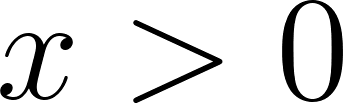 . Write the call using the differentiable operators, choosing the right
 :support. What is the Jacobian contribution, and why is it the same as for any latent?
Problem 11.7 (A new model). Using the existing distributions and the DSL, write a for a Poisson rate:  prior, and
  a vector of count data with
 (poisson lambda). Generate  counts from a Poisson with true rate
  , fit the model with HMC and two chains, and check that the posterior mean of
 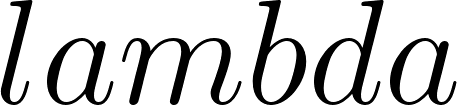 covers . Compare with the exact Gamma posterior from Chapter 9’s conjugacy (Gamma-Poisson).
Problem 11.8 (Comparing engines). Fit the regression model with all three engines (:mh, :hmc, :vi), two chains each where supported. For each engine, report the posterior mean of  , the ESS, and the wall-clock time (use
  around the call). Rank the engines by accuracy and by speed. Which engine gives the best tradeoff for this three-parameter model?
Problem 11.9 (Variational bias). The three-engine table shows variational inference with a larger error than the two samplers. The variational guide is a factorized Normal in unconstrained space, transformed by the sigmoid. Explain in your own words why the mean of  with
with  is not
 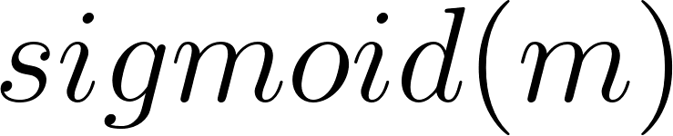 , and why this introduces a bias that grows with the variance
 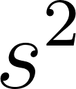 . Suggest one way to reduce the bias (for example, fitting on the natural scale, or using a Beta guide).
Problem 11.10 (Coding exercise). The HMC engine uses a fixed, jittered path length. Replace it with a simple doubling scheme: start with one leapfrog step, and double the path length while the proposed Hamiltonian energy decreases, stopping at a maximum or when the energy starts to rise. This is a simplified version of the No-U-Turn condition. Test your modified engine on the regression model and report the effect on ESS and acceptance rate compared with the fixed-path-length version.