Bayesian Inference
In the chapter on conditional probability we encountered Bayes’ theorem as a way to reverse the direction of conditioning. Bayesian inference extends this idea to a full framework for learning from data. We start with a belief about an unknown parameter, then update that belief as evidence arrives.
The example program for this chapter is in the file 09_bayesian_inference.lisp.
Two Paradigms of Statistics
Statistical inference broadly divides into two paradigms: frequentist and Bayesian. Understanding the difference is important because they answer subtly different questions.
The frequentist view treats a parameter as an unknown but fixed constant. The data are random, and any statement about the parameter must be phrased in terms of the sampling distribution of an estimator. A frequentist 95% confidence interval means: if the experiment were repeated many times, 95% of the intervals we construct this way would contain the true parameter. It says nothing directly about the probability that the specific interval we computed contains the true value.
The Bayesian view treats the parameter itself as a random variable with a probability distribution that expresses our belief. Data are observed, but the parameter distribution is what we update. A Bayesian 95% credible interval means: given the data, there is a 95% probability that the parameter lies in the interval, under our prior beliefs.
Neither paradigm is universally “correct”; they are two different frameworks for reasoning under uncertainty. Bayesian methods are natural when we have meaningful prior information or when we want to make direct probability statements about parameters. Frequentist methods can be more objective when there is disagreement about the prior. In modern practice, most working statisticians and machine-learning engineers use both, choosing the paradigm that best fits the problem at hand.
The Bayesian Framework
In Bayesian inference, an unknown parameter 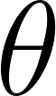 is treated as a random variable with its own probability distribution. The core equation is:

Reading from right to left:
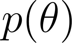 is the prior: what we believe about before seeing any data.
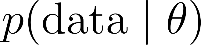 is the likelihood: how likely the observed data is if has a particular value.
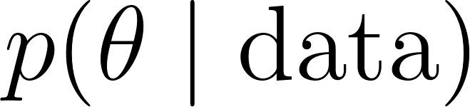 is the posterior: what we believe about after seeing the data.
The proportionality constant is 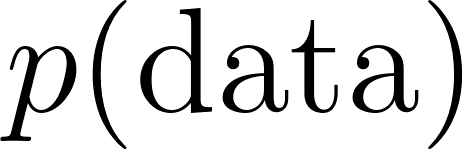 , which normalizes the posterior so it sums (or integrates) to
  . In practice, we often work with the unnormalized posterior and normalize at the end.
The posterior distribution is the complete answer that a Bayesian inference provides. From it we can compute point estimates (like the posterior mean or median), credible intervals, and predictions about future data. The posterior is a much richer object than a single point estimate; it captures how much we know and how much we still do not know.
The Choice of Prior
The prior expresses beliefs about theta before observing data. In some problems, we have genuine prior information (from previous studies, physical constraints, or expert opinion), and the prior encodes that. In other problems, we want the data to speak for itself and use an uninformative prior.
Several classical choices of uninformative prior appear in the literature:
- Uniform prior: assign equal density to all values of. This is what we use in the example (
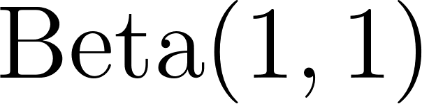 ) for a coin bias. Uniform priors seem to convey no information, but they are not invariant under reparameterization: a uniform prior on the probability
  is not uniform on the odds
 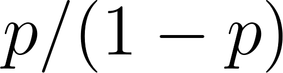 .
.
- Jeffreys prior: constructed to be invariant under reparameterization. For a Bernoulli likelihood, the Jeffreys prior is
 , which is peaked near
 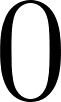 and .
and .
- Reference priors: derived to maximize the information gain from the data, again invariant under transformations.
The choice of uninformative prior can matter for small sample sizes but usually washes out as more data arrive. This convergence of the posterior toward the true value regardless of the prior is one of the most attractive features of Bayesian inference.
The prior can also express strong beliefs. In a clinical trial with a new drug, a prior might reflect the fact that most new drugs do not work well; this “skeptical” prior would then require substantial evidence in the data before concluding that the drug is effective. This is not cheating; it is a principled way to incorporate what we already know.
Conjugate Priors
For certain combinations of likelihood and prior, the posterior is in the same family as the prior. This is called conjugacy, and it makes Bayesian updating remarkably simple.
For a Bernoulli or binomial likelihood with unknown success probability , the conjugate prior is the Beta distribution. If the prior is 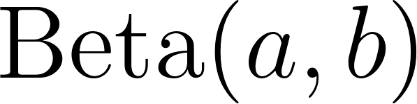 and we observe
  successes and
 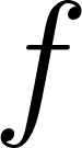 failures, the posterior is:

The distribution has a density on the interval 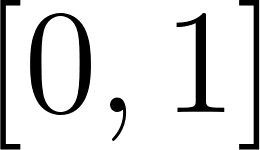 :
:
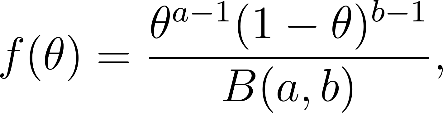
where 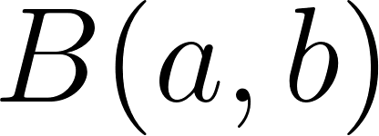 is the Beta function (the normalizing constant). The parameters
  and
and 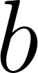 act as pseudo-counts:
 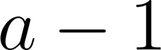 prior successes and
 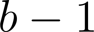 prior failures.
The conjugacy is a one-line calculation. The likelihood of successes and failures is  , and the prior density is proportional to
  . Multiplying them,

which is the unnormalized  density. The two factors have the same functional form in , so their product stays in the Beta family; only the exponents move. This is exactly why the update is just addition of counts, and why we never need to touch the awkward normalizing constant while updating.
The mean and variance are:

The program implements these formulas:
1 (defun beta-mean (a b)
2   "Posterior/prior mean of Beta(a,b): E[theta] = a / (a + b)."
3   (/ a (+ a b)))
4
5 (defun beta-variance (a b)
6   "Var(theta) for Beta(a,b): a b / ((a+b)^2 (a+b+1))."
7   (/ (* a b) (* (expt (+ a b) 2) (+ a b 1))))
Other Conjugate Pairs
Beta and Bernoulli are not the only conjugate pair. Several others show up frequently:
- Normal-Normal: if the data are normal with unknown mean but known variance, and the prior on the mean is normal, then the posterior on the mean is also normal.
- Gamma-Poisson: if the data are Poisson counts with unknown rate, and the prior on the rate is Gamma, then the posterior is also Gamma.
- Dirichlet-Multinomial: the multivariate generalization of Beta-Bernoulli, used for categorical distributions with more than two outcomes.
These pairs are not a coincidence. A conjugate prior exists whenever the likelihood belongs to an exponential family, the class of distributions whose density can be written as  for a natural parameter
  , a sufficient statistic
 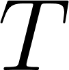 , and a log-partition function
 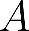 . The Bernoulli, Poisson, normal, and multinomial are all exponential families, which is why each has a tidy conjugate partner. The conjugate prior is built to share the algebraic form of the likelihood in , so that multiplying prior by likelihood updates the parameters and leaves the shape untouched. The sufficient statistic
 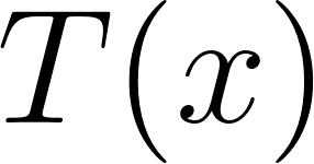 is what the pseudo-counts accumulate: for the Bernoulli it is the success count, which is why our update simply adds and .
Conjugacy is a mathematical convenience: it lets us do inference in closed form. In modern practice, however, we rarely have neat conjugate models. Bayesian inference in complex models usually uses Monte Carlo methods (Markov chain Monte Carlo, variational inference) to approximate the posterior. But conjugate models remain valuable for building intuition and as building blocks in larger hierarchical models.
The Update Rule
The beauty of conjugacy is that the update rule is just addition. Each observed success increments a, and each observed failure increments b:
1 (defun bayesian-update (prior-a prior-b successes failures)
2   "Conjugate update for a Beta prior with Bernoulli/binomial data.
3    Prior  Beta(a, b)  ->  Posterior Beta(a + s, b + f)."
4   (values (+ prior-a successes) (+ prior-b failures)))
This is the same result whether we update all at once (batch) or one observation at a time (sequential). Conjugacy guarantees that the final posterior is the same either way. This equivalence of batch and sequential updating is a very useful property; it means we can process data as it arrives without waiting for it all to be collected.
The Posterior Mean as a Weighted Average
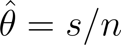
The conjugate update has an interpretation that explains the prior-sensitivity behaviour we return to later. Write the prior mean as  and the sample proportion, which is the maximum-likelihood estimate, as
  with
with 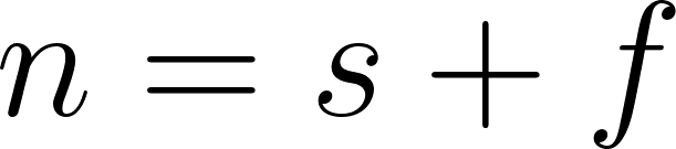 . The posterior mean rearranges into a convex combination:

The posterior mean sits between the prior mean and the data’s own estimate, with weights set by the prior strength 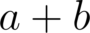 and the sample size
  . The Bayesian estimate is shrunk from the raw proportion toward the prior mean. When data are scarce (
 ) the prior dominates; when data are plentiful (
 ) the weight on the prior fades like
 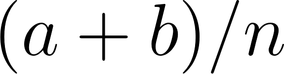 and the estimate reduces to the sample proportion. This one formula is the precise sense in which “the prior washes out,” and it justifies reading as a count of prior observations that compete on equal footing with the real ones.
Point Estimates and Credible Intervals
The posterior distribution is the complete answer, but sometimes we want a single number or a range as a summary.
The posterior mean 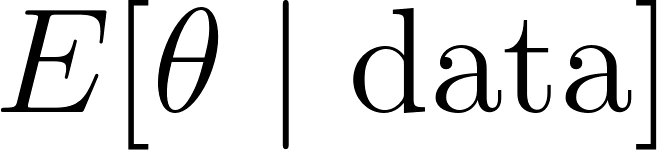 is the standard point estimate. It minimizes squared-error loss.
The maximum a posteriori (MAP) estimate is the value of that maximizes the posterior density. It corresponds to the “mode” of the posterior. When the prior is flat, the MAP estimate coincides with the maximum-likelihood estimate.
A credible interval is a range that contains the parameter with a specified posterior probability. A 95% credible interval 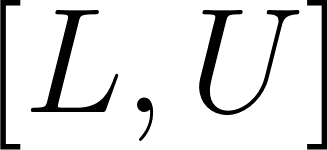 satisfies
  . Credible intervals answer the question that most practitioners really want: given what I have observed, what is a plausible range for the parameter?
Prediction: The Posterior Predictive
Bayesian inference gives more than parameter estimates; it also gives principled predictions about future data. The posterior predictive distribution for a future observation 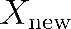 given past data
  is:
is:

This averages the likelihood over the posterior on . Unlike a frequentist point-prediction, the posterior predictive automatically accounts for uncertainty in .
For the Beta-Bernoulli model, if the posterior after observations is , then the probability of a success on the next trial is  . This is exactly the posterior mean, which is why the posterior mean is such a natural point estimate.
The Example: Estimating a Coin’s Bias
We start with a prior, which is the uniform distribution on . This represents maximum ignorance: before seeing any data, every value of is equally likely.
Then we simulate 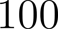 flips of a coin with true bias
 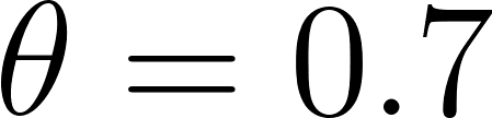 and update our posterior. The program shows the posterior at several intermediate stages:
 1 (defun main ()
 2   (let ((prior-a 1) (prior-b 1))      ; Beta(1,1) = Uniform(0,1)
 3     (print-beta prior-a prior-b "Prior         ")
 4     (let* ((rs (make-random-state t))
 5            (data (loop for i below 100
 6                        collect (if (< (random 1.0d0 rs) 0.7d0) 1 0))))
 7       (let ((successes (count 1 data))
 8             (failures (count 0 data)))
 9         (multiple-value-bind (pa pb) (bayesian-update prior-a prior-b
10                                                        successes failures)
11           (print-beta pa pb "Posterior     "))
12         ;; Show intermediate stages
13         ...))))
Running the Example
 1 === Bayesian Inference for a Coin Bias ===
 2 Likelihood: Bernoulli(theta). Prior: Beta(1,1) = Uniform on [0,1].
 3 True theta (used only to generate data) = 0.7.
 4
 5   Prior         : Beta(1, 1)  mean= 0.5  var=0.0833
 6
 7 Observed 74 successes and 26 failures in 100 flips.
 8   Posterior     : Beta(75, 27)  mean=.735  var=0.0019
 9
10 Sequential updates (belief concentrates as data arrives):
11   After 10   flips: Beta(8, 4)  mean=.667  var=0.0171
12   After 50   flips: Beta(37, 15)  mean=.712  var=0.0039
13   After 100  flips: Beta(75, 27)  mean=.735  var=0.0019
14
15 True theta = 0.7. As n grows the posterior mean converges to the
16 true value and the variance shrinks to 0 (Bernoulli's theorem).
Because the program simulates fresh coin flips on each run, the exact counts and posterior values here are one representative realization. Your numbers will differ, but the pattern is the same every time: the posterior mean drifts toward 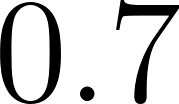 and the variance shrinks.
Watch what happens as data accumulates:
- Prior: with mean
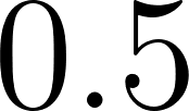 and variance
 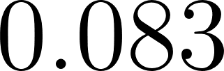 . We know nothing yet.
- After
10$ flips: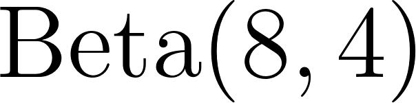 with mean
 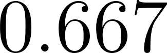 and variance
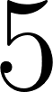
 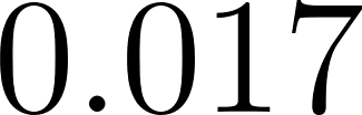 . The mean has shifted toward , and the variance has shrunk by a factor of
  .
.
- After
50$ flips: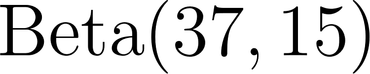 with mean
 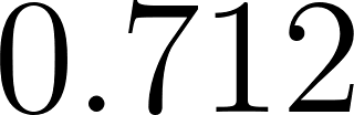 and variance
 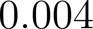 . We are getting closer, and the variance is still shrinking.
- After
100$ flips: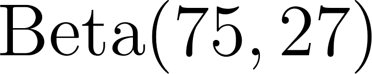 with mean
 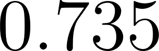 and variance
 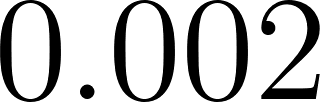 . The posterior mean is close to the true value of , and the variance is tiny.
The posterior mean () is not exactly because we only have data points. With 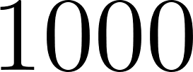 flips, it would be even closer. The variance continues to shrink toward zero as more data arrives, reflecting increasing confidence in our estimate.
The Laplace Rule of Succession
With a uniform prior , the posterior mean after successes and failures is:
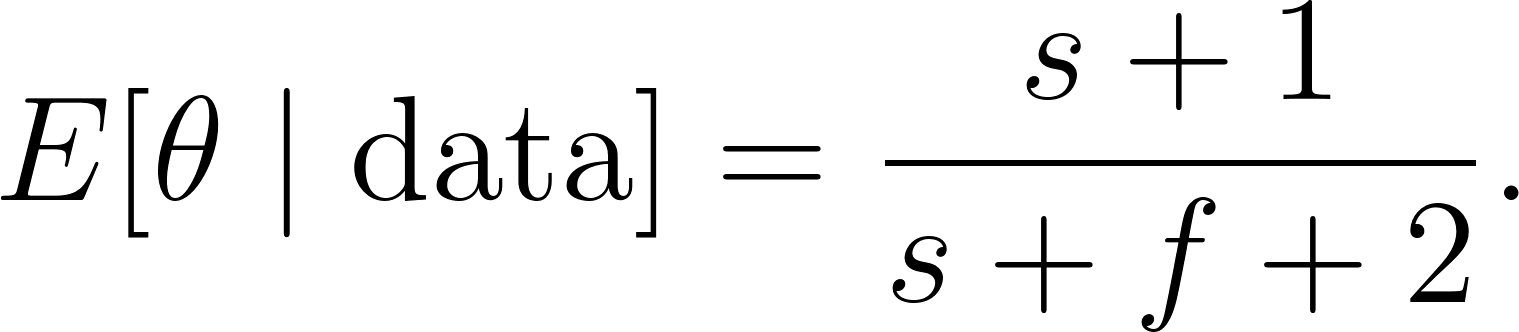
This is the famous Laplace rule of succession. If you have seen successes in 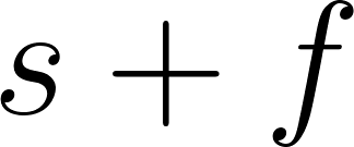 trials, your best estimate of the success probability is
  , not
, not 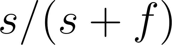 . The
. The 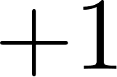 and
and 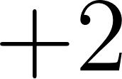 come from the prior pseudo-counts. This rule prevents overconfidence from small samples: if you flip a coin once and get heads, the rule estimates the bias as
 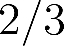 rather than .
Laplace himself used this rule to estimate the probability that the sun would rise tomorrow given that it has risen every day so far. The result is silly if taken too literally, but the underlying mathematical idea, that small samples should not be treated as certain, is enduring and important.
Prior Sensitivity
An important practical question is how much the choice of prior affects the posterior. The general answer is: for small data, the prior matters a lot; for large data, it washes out.
To see this concretely, compare the posterior mean after successes in trials for two different priors:
- prior: posterior mean

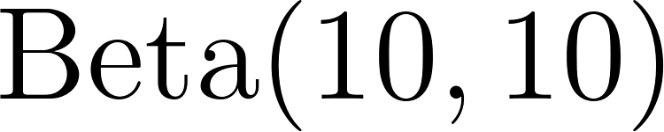 prior: posterior mean
For 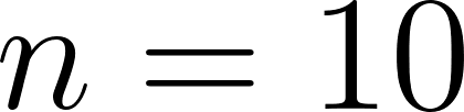 and
and 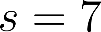 , the first gives
  , and the second gives
  . These are quite different. But for
  and
and  , the first gives
  , and the second gives
  . They are essentially the same. This washout effect is a hallmark of Bayesian inference with lots of data.
Why This Matters
Bayesian inference is the foundation of modern machine learning in many domains. Spam filters use it to classify emails. Medical tests use it to interpret results. A/B testing platforms use it to decide which variant is better. Recommendation systems use it to model user preferences.
The key insight of Bayesian inference is that learning is the process of updating beliefs. You start with what you know (the prior), you observe data (the likelihood), and you update your knowledge (the posterior). This cycle can be repeated indefinitely: each posterior becomes the prior for the next round of data. As data accumulates, the posterior concentrates around the true value, and the prior’s influence fades away. This convergence is guaranteed by Bernoulli’s theorem, a special case of the Law of Large Numbers applied to the posterior distribution.
Problem Set
Problem 9.1. Starting from a prior and observing 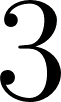 successes in
 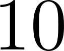 flips, compute the posterior parameters, the posterior mean, and the posterior variance. Compare with the raw sample proportion
 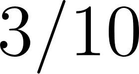 .
.
Problem 9.2 (Sequential vs. batch). Observe the sequence of coin flips 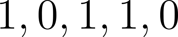 . Starting from , update the posterior after each flip and record the
 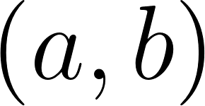 pair at each step. Then compute the batch update after all flips. Verify that the two answers agree.
Problem 9.3 (Prior sensitivity). Suppose the data are 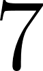 successes in trials. Compute the posterior mean for three priors:
  , and
, and 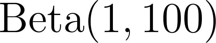 . Interpret each of these priors in words and explain how they influence the posterior estimate.
Problem 9.4 (Credible interval). For a posterior, compute an approximate 95% credible interval . Since the Beta CDF is not elementary, use numerical integration of the density (as the example program does for normalization) and find the values 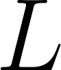 and
and 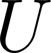 such that
  and
and  .
.
Problem 9.5 (MAP estimate). For a distribution with 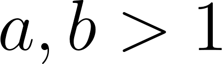 , the mode is at
  . Verify this by differentiating the log-density and setting the derivative to zero. Compute the MAP estimate for a posterior and compare with the posterior mean.
Problem 9.6 (Posterior predictive). For a posterior, what is the probability that the next flip is heads? Now compute the probability that the next two flips are both heads. Hint: the answer is not 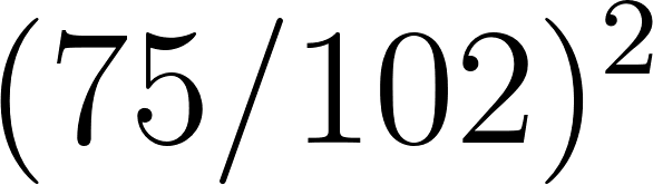 . Use the fact that the two flips are not independent given the posterior on ; average the joint likelihood over the posterior.
Problem 9.7 (Jeffreys prior). Rerun the example with a prior instead of . Compare the posterior after flips ( successes, failures) under both priors. When do the two priors give noticeably different answers?
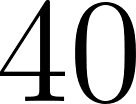
Problem 9.8 (A biased coin). Suppose you have strong prior belief that a coin is fair, expressed as a 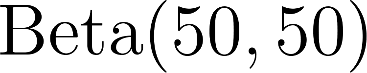 prior (mean and quite concentrated). You then observe
 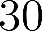 heads in
  flips. What is your posterior mean? Is the data enough to override your prior?
Problem 9.9 (Coding exercise). Extend the example program to compute the posterior predictive probability of the next observation being a success. Also extend it to plot (or print a text histogram of) the posterior density at several intermediate stages so you can visually watch the belief concentrate.
Problem 9.10 (A different conjugate pair). Suppose you are counting the number of shooting stars per hour and model it as 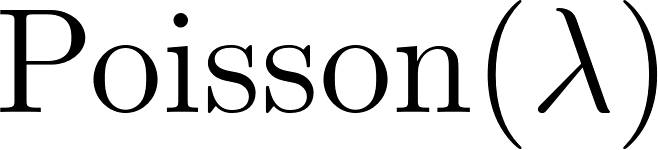 . A conjugate prior for the rate
 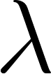 is
is  , and the posterior after observing counts
  is
is  . Starting from a
  prior and observing counts
 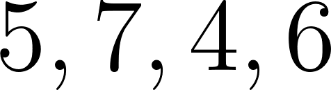 , compute the posterior parameters and the posterior mean. Compare with the sample mean of the counts.