Basic Probability

Probability theory begins with a simple but powerful idea: we can assign numbers between 0 and 1 to events to measure how likely they are. This chapter introduces the fundamental vocabulary of probability theory and the three axioms that everything else is built upon.

The example program for this chapter is in the file 01_basic_probability.lisp.

The mathematical study of probability grew out of very practical questions. In the sixteenth century the Italian polymath Gerolamo Cardano wrote Liber de Ludo Aleae (The Book on Games of Chance), analyzing dice games and card games with an eye toward gambling strategy. In 1654 the French mathematicians Blaise Pascal and Pierre de Fermat exchanged a famous series of letters about the “problem of points”: how should the stakes be divided if a game of chance is interrupted before it is finished? Their correspondence is often cited as the birth of probability theory as a mathematical discipline.

Over the next three centuries, Jakob Bernoulli, Abraham de Moivre, Pierre-Simon Laplace, Carl Friedrich Gauss, Pafnuty Chebyshev, and many others developed probability into a sophisticated body of theory. But for a long time the field lacked rigorous foundations. Different authors used different definitions, and paradoxes appeared whenever the intuitive notion of “probability” was pushed hard enough.

In 1933 the Russian mathematician Andrey Kolmogorov published a short monograph, Grundbegriffe der Wahrscheinlichkeitsrechnung (Foundations of the Theory of Probability), that finally put probability on firm mathematical footing. He grounded it in measure theory and reduced its foundations to just three axioms. Everything we do in this book, and everything in modern probability theory, ultimately traces back to Kolmogorov’s axioms.

Before we plunge into the mathematics, it is worth pausing to ask: what does a probability actually mean? There are several answers, and they are not always in conflict.

The classical interpretation, associated with Laplace, says that if there are equally likely outcomes and 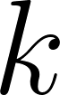of them are favorable to some event, then the probability of the event is 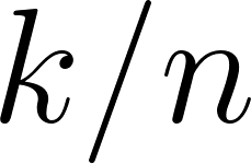. This is the interpretation used when we say a fair die has probability 1/6 of showing a 4. It works well for games of chance where symmetry gives us equally likely outcomes for free.

The frequentist interpretation says that the probability of an event is the long-run fraction of times it occurs in repeated trials. If we flip a coin ten thousand times and see 4,972 heads, we would estimate the probability of heads as roughly 0.4972. This interpretation grounds probability in observable frequencies and is the philosophical basis for much of classical statistics.

The subjective (or Bayesian) interpretation treats probability as a degree of belief. Under this view, it is meaningful to talk about the probability that a particular historical event happened, or the probability that a specific hypothesis is true, even if there is no notion of “repeated trials.” Bayesians update their beliefs using Bayes’ theorem as new evidence arrives.

The remarkable thing about the Kolmogorov axioms is that they are compatible with all three interpretations. The mathematics works the same way regardless of which interpretation you prefer, and each interpretation illuminates different applications.

A random experiment is any procedure whose outcome we cannot predict with certainty. Flipping a coin, rolling a die, and drawing a card from a deck are all random experiments.

The sample space, written , is the set of all possible outcomes of a random experiment. When we roll a single die, the sample space is . When we roll two dice, the sample space consists of all 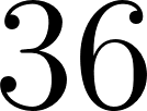ordered pairs 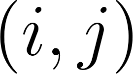where and range from to .

An event is any subset of the sample space. When rolling two dice, the event “the sum is 7” is the set of all outcomes where the two dice add up to . There are such outcomes: , and .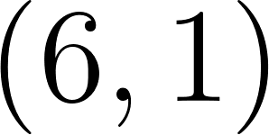

Note that events are just sets of outcomes. The distinction between an outcome (a single element of ) and an event (a subset of ) is important. The outcome 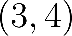is a single point of the sample space; the event “the first die is 3” is the six-element set . A single outcome can also be viewed as a singleton event, but not every event corresponds to a single outcome.

In the example program, we build the sample space for two dice as a list of all 36 ordered pairs:

The events are defined by filtering the sample space with a predicate. For example, the event “sum equals 7” keeps only the outcomes where the two dice add up to 7:

Because events are sets, we can combine them using set operations, and each operation has a natural probabilistic meaning:

• Union : the event that or (or both) occurs. In Lisp we compute it with union.
• Intersection : the event that both and occur. In Lisp we compute it with intersection.
• Complement (or “not A$”): the event that does not occur. Its outcomes are those in but not in .
• Difference 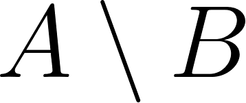: the event that occurs but does not. It equals .

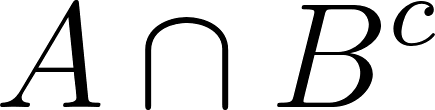Two events are called disjoint (or mutually exclusive) if their intersection is empty. Disjoint events cannot both happen at the same trial. For example, “sum equals 7” and “sum equals 11” are disjoint events on the two-dice sample space.

De Morgan’s laws connect complementation to union and intersection:

In words, “not (A$ or B$)” is the same as “not A$ and not B$,” and “not (A$ and B$)” is the same as “not A$ or not B$.” These laws are extraordinarily useful when you find it easier to reason about complements.

So far we have said that an event is any subset of . For a finite sample space such as the 36 outcomes of two dice, that statement causes no trouble: we take every subset to be an event, and there are 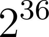of them. When the sample space is uncountable, though (for example the real line, which we meet in the chapter on continuous distributions), we cannot consistently assign a probability to every subset. Measure theory shows that pathological, non-measurable sets exist, and forcing a probability onto them breaks countable additivity. The fix is to name in advance the collection of subsets we agree to call events, and to require only that this collection stay closed under the operations we care about.

Such a collection is a \sigma$-algebra (sigma-algebra) on . It must satisfy three closure properties:

1. : the whole space is an event.
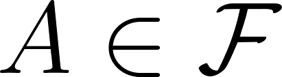2. If then : closed under complement.
3. If then 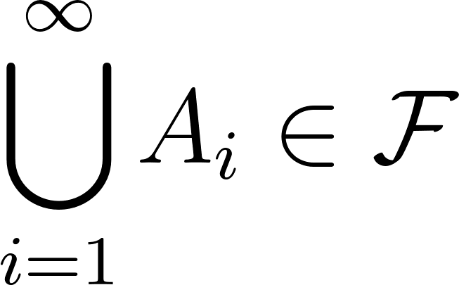: closed under countable union.

Closure under countable intersection then follows from De Morgan’s laws. The pair 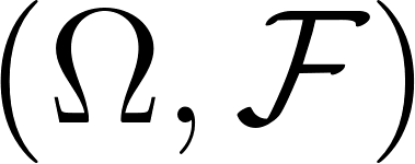is a measurable space, and the sets in are the events. A probability measure is a function on the event space, , not on arbitrary subsets. The three ingredients together,

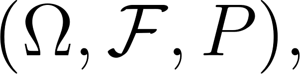
form a probability space, or probability triple. Every model in this book is a probability space, even where we do not write it out.

For a finite or countable sample space we always take to be the collection of all subsets, the power set 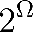, and the subtlety disappears. This covers every discrete example in the book. The machinery matters only when is uncountable, where the standard choice is the Borel \sigma$-algebra: the smallest -algebra that contains all the open intervals. We name it now so that the word “event” has a precise meaning when we reach continuous distributions.

In 1933, the Russian mathematician Andrey Kolmogorov formulated three axioms that serve as the foundation of modern probability theory. A probability measure is a function that assigns a number to each event, satisfying these three rules:

1. Non-negativity: 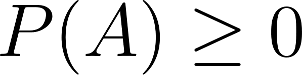for every event . Probabilities are never negative.
2. Normalization: 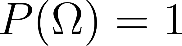. The probability of the entire sample space is , meaning that some outcome must occur.
3. Countable additivity: If are pairwise disjoint events (no two of them share an outcome), then .

These three axioms are remarkably compact, yet they generate the entire edifice of probability theory. Every theorem we will encounter in this book can be traced back to these three statements.

Why countable, and not merely finite, additivity? Axiom 3 is stated for an infinite sequence of disjoint events, not just for a finite collection. Finite additivity, 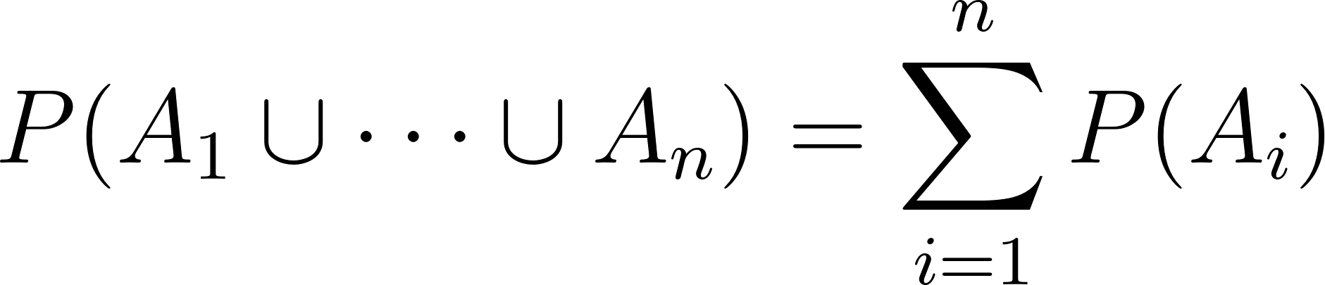, is the special case in which all but finitely many 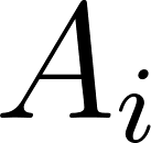are empty. The stronger countable version is what lets us pass to limits. It guarantees, for instance, that if a sequence of events shrinks toward the empty set then their probabilities shrink toward zero. Without this continuity we could not build the convergence theorems, the Law of Large Numbers and the Central Limit Theorem, that occupy the later chapters. Finitely additive measures do exist and are studied in their own right, but they lack the limiting behaviour that makes probability useful.

Several important properties follow immediately from the three axioms. Each one is worth internalizing because we will use them constantly.

Probability of the empty set is zero. Since and the empty set are disjoint and their union is , by additivity , so .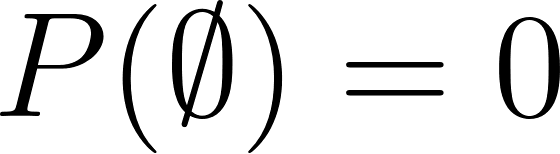

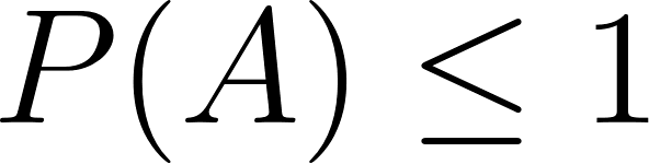
Probabilities are bounded above by 1. Since and its complement are disjoint and their union is , we have . Non-negativity of 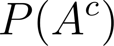forces . Combining with axiom 1, every probability lies in the interval .

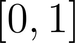Complement rule. As already noted, . This is often the fastest way to compute a probability when the direct calculation is awkward.

Monotonicity. If 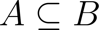, then . This says that adding outcomes to an event can only make it more likely, which matches intuition.

Inclusion-exclusion for two events. For any events and :

The term 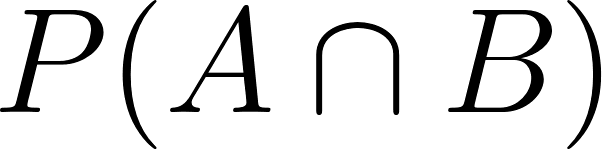corrects for double-counting the outcomes that lie in both events. For events the pattern continues, alternating signs across intersections of every size:

Truncating this sum after any term yields the Bonferroni inequalities. Stop after the first sum and you get the union bound below; stop after the second and you get a lower bound; each further term tightens the estimate, and the partial sums bracket the true probability from alternating sides. These bounds are the everyday tool for controlling the probability of a union when the higher-order intersection terms are hard to compute.

Subadditivity (Boole’s inequality). For any events and , whether disjoint or not:

More generally, 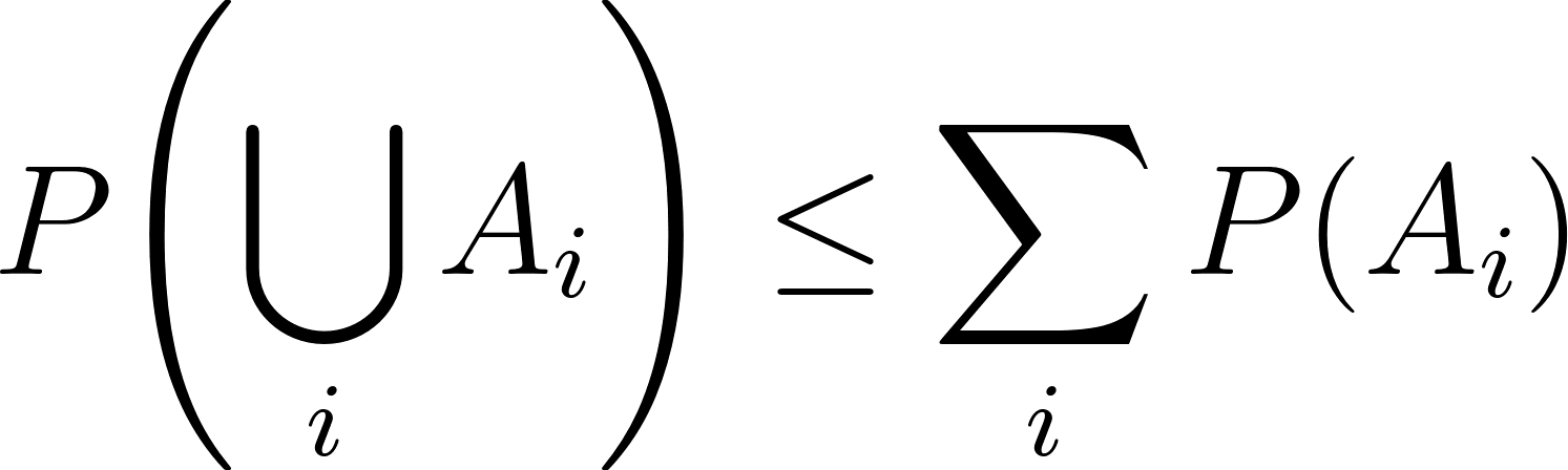: the probability of a union is at most the sum of the individual probabilities. This is the union bound, and it is one of the most heavily used inequalities in the probabilistic analysis of algorithms, where one bounds the chance that any of many rare failures occurs by summing their individual chances.

Continuity of probability. Countable additivity is equivalent to a continuity property. If events increase to a limit, with union , then . Likewise if events decrease, with intersection , then . We lean on this quietly every time we take a limit of probabilities, which in the later chapters is often.

When all outcomes in the sample space are equally likely, the probability of an event reduces to a simple counting problem:

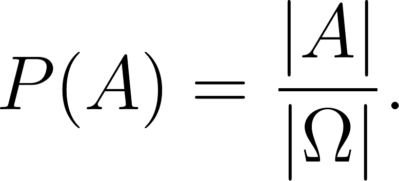
That is, the probability of event is the number of favorable outcomes divided by the total number of outcomes. This is called the classical definition of probability, and it is what most people learn first.

In the language of the event space above, the classical definition is one particular probability measure on a finite space: the uniform measure, which places equal mass 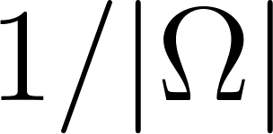on each outcome. It is a special case, not the general rule. It presupposes that the outcomes really are equally likely, which some symmetry of the experiment justifies (a fair die, a well-shuffled deck) but which fails the moment the symmetry breaks. A loaded die still has sample space 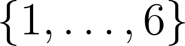, yet its six probabilities are not all 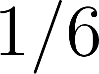. For a general discrete model we assign a mass 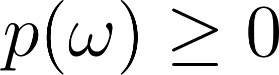to each outcome with 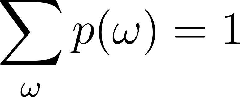, and recover the probability of an event by summing the masses it contains:

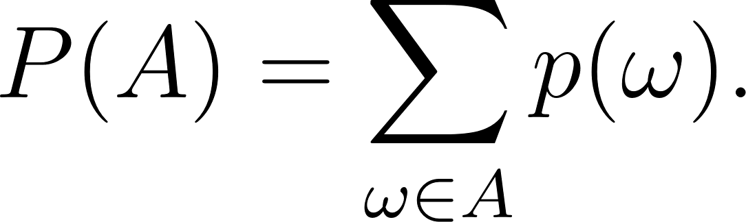
The classical formula is the case where every 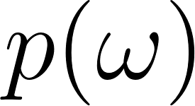equals . We meet the general form again in the next chapter as the probability mass function of a random variable.

For two fair dice, each of the 36 outcomes is equally likely, so we can compute probabilities by counting:

The function returns an exact rational number. Lisp’s rational arithmetic is a nice fit for probability calculations because many probabilities are fractions like 1/6 or 11/36.

The classical formula reduces every problem to counting. Two combinatorial tools appear again and again:

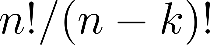
Permutations count ordered arrangements. The number of ways to arrange distinct objects in a row is ( factorial). The number of ordered arrangements of objects chosen from is .

Combinations count unordered selections. The number of ways to choose objects from distinct objects without regard to order is the binomial coefficient 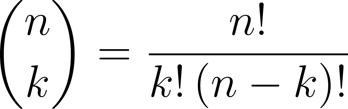. We will meet the binomial coefficient again in the chapter on the binomial distribution.

For the two-dice sample space, no combinatorial machinery is needed: the sample space has exactly elements, one for each ordered pair. But in a card problem, or in a problem involving many coin flips, you almost always start by counting the sample space with permutations or combinations.

A direct consequence of the axioms is the complement rule:

This follows because an event and its complement (everything in the sample space that is not in ) partition the sample space. By the additivity axiom, , so .

The complement rule is surprisingly useful. Sometimes it is easier to compute the probability that something does NOT happen, and then subtract from 1. For example, the probability of rolling “at least one 6” in two dice is easier to compute via its complement “no 6 appears at all”:

When you load the program, it builds the two-dice sample space and computes several probabilities:

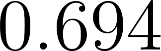
Notice that , confirming the normalization axiom. The probability of rolling a sum of is , which makes sense because there are favorable outcomes out of . The complement rule gives us , which is approximately .

The concepts in this chapter may seem simple, but they are the foundation for everything that follows. Conditional probability, random variables, distributions, and the great theorems of probability all build on the ideas of sample spaces, events, and the Kolmogorov axioms. When you find yourself confused by a more advanced concept, returning to these foundations often clears things up.

The problems below give you a chance to apply the ideas of this chapter. All of them can be solved on paper, but I encourage you to also verify your answers by extending the Common Lisp program. Building the sample space and filtering by a predicate is a very general recipe that works for many discrete probability problems.

Problem 1.1. For the two-dice sample space, compute and . Verify that they add to , as the axioms require.

Problem 1.2. Let be the event “the first die is 3” and be the event “the sum is 5.” Compute , and 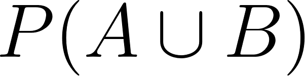directly. Then verify the inclusion-exclusion formula .

Problem 1.3. Compute the probability that at least one die shows an even number. Do this two ways: (a) directly by counting outcomes, and (b) via the complement rule using the event “both dice are odd.” Confirm the answers agree.

Problem 1.4. Extend the program to three dice. The new sample space has 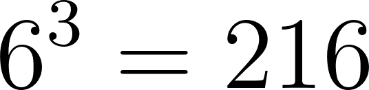outcomes. Compute the probability that the sum is exactly . (For those who want to check by hand, the answer is .)

Problem 1.5. Draw a card from a standard 52-card deck. Let be the event “the card is a heart” and be the event “the card is a face card (jack, queen, or king).” Assuming all 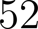cards are equally likely, compute , and . Are and disjoint? Explain.

Problem 1.6. A fair coin is flipped times. Using the classical definition, what is the probability of getting exactly 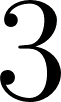heads? Hint: the sample space has 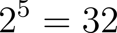outcomes, and the number of ways to arrange heads among flips is the binomial coefficient . Now compute the probability of “at least 3 heads” and the probability of “at most 3 heads,” and use these to check the complement rule.

Problem 1.7 (De Morgan in action). For any two events and on any sample space, prove that . Then use this identity to give an alternative derivation of the inclusion-exclusion formula.

Problem 1.8 (Coding exercise). Modify the example program to accept an arbitrary predicate and print (a) the number of favorable outcomes, (b) the probability as an exact rational, and (c) the probability as a decimal. Then use this generalized reporter to compute the probability that the two dice differ by exactly .