Central Limit Theorem

The Law of Large Numbers tells us that the sample mean converges to the true mean. But it does not tell us how the sample mean is distributed around that mean. The Central Limit Theorem (CLT) answers this question, and its answer is one of the most remarkable results in all of mathematics: the distribution is approximately normal, no matter what the original distribution looks like.

The example program for this chapter is in the file 07_central_limit_theorem.lisp.

The Central Limit Theorem has a long and distinguished history. The earliest form was proved by Abraham de Moivre in 1733 for the special case of Bernoulli trials: he showed that the binomial distribution is well approximated by a normal distribution for large n. Pierre-Simon Laplace generalized De Moivre’s result in his monumental Theorie Analytique des Probabilites (1812) and applied it to problems in astronomy and geodesy, where he needed to reason about the distribution of averaged measurement errors.

The modern general form of the CLT, allowing arbitrary distributions with finite variance, was proved by the Russian mathematician Aleksandr Lyapunov in 1901. Later, the theorem was refined to handle non-identically-distributed variables under a technical condition known as the Lindeberg condition. Even today, generalizations of the Central Limit Theorem are an active area of research, especially for weakly dependent variables and high-dimensional problems.

Let 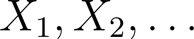be i.i.d. random variables with mean and finite variance 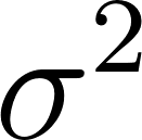. Let be their sum. The CLT says that for large , the standardized sum:

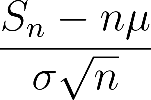
converges in distribution to the standard normal distribution .

Equivalently, the sample mean 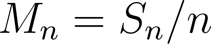is approximately for large . Notice that the variance of 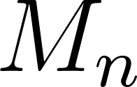shrinks as 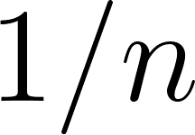: more data means a tighter distribution around the mean. But the CLT tells us more than the LLN did: it tells us the shape of the distribution of , not just that it concentrates.

Written as a limit of CDFs, the CLT says:

where is the CDF of the standard normal. This mode of convergence is called convergence in distribution or weak convergence. It is the weakest of the modes we surveyed in the previous chapter, and even so, it delivers enormous practical value.

The CLT says that the original 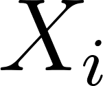can have any distribution with finite variance, and the sum will still become approximately normal. The could be Bernoulli, uniform, exponential, or some weird custom distribution. It does not matter. Sums of enough i.i.d. random variables always tend toward the normal distribution.

This is why the normal distribution appears everywhere in nature. Many natural quantities are sums or averages of many small independent effects. Heights, measurement errors, blood pressure, and countless other quantities are approximately normal because they are built from the sum of many independent contributions.

The result is worth savoring. A theorem that starts with almost no assumptions about the except finite variance ends with a very specific conclusion: the standardized sum is a standard normal. It is almost as if the normal distribution is the mathematical shadow of independence and averaging.

The moment generating function from Chapter 3 gives a clean way to see why the normal appears, not just that it does. Standardize the individual variables by writing , so each 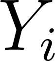has mean and variance . The standardized sum is

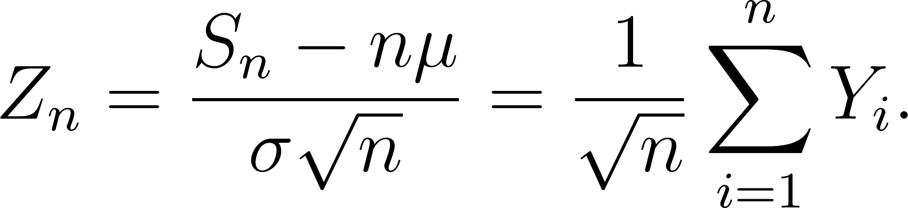
Because the are independent, the MGF of 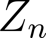is the -th power of one scaled MGF:

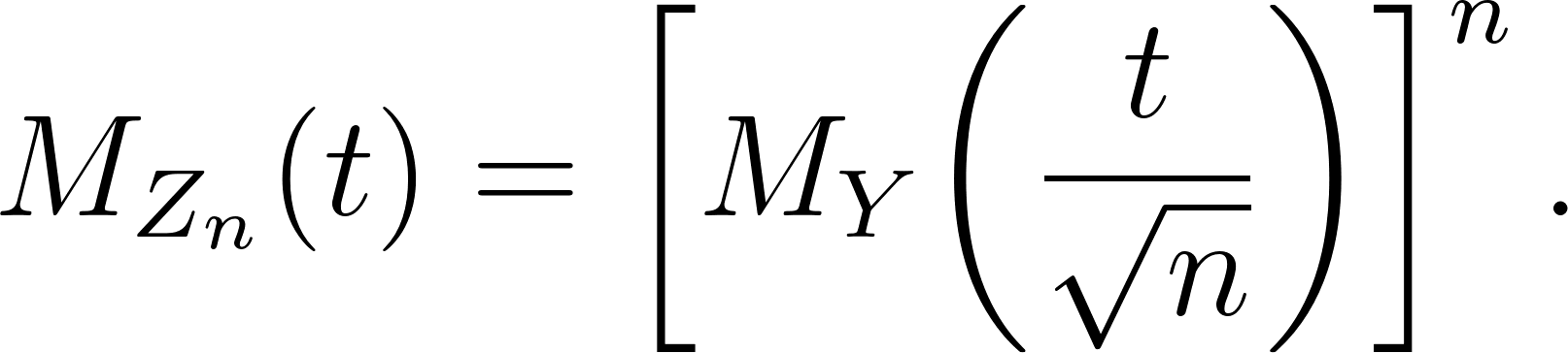
Now expand 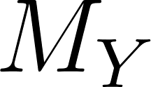near . Since 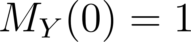, , and , the Taylor expansion is . Substituting 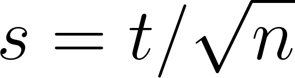and raising to the -th power,

The limit 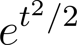is exactly the MGF of the standard normal (set 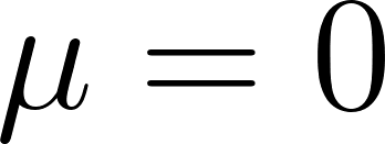, 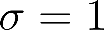in the normal MGF of Chapter 5). Since the MGF determines the distribution, converges to . The whole theorem comes down to one fact: only the first two moments survive the 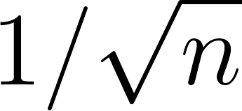scaling. Every distribution with finite variance has the same quadratic leading behaviour, so they all flow to the same bell curve. The 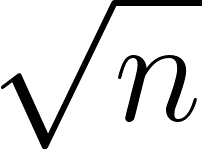in the denominator is forced, being the unique scaling that holds the variance of at ; divide by and you get the constant of the Law of Large Numbers, divide by less and the variance blows up. A fully rigorous proof replaces the MGF with the characteristic function , which exists for every distribution, but the algebra is the same.

The plain CLT is a limit statement: it does not tell us how large has to be for the normal approximation to be accurate. The Berry-Esseen theorem provides a quantitative bound. Under the additional assumption that the have finite third absolute moment 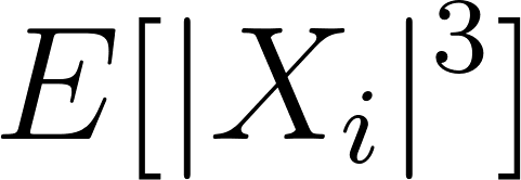, the maximum difference between the CDF of the standardized sum and the standard normal CDF satisfies:

for some absolute constant (the best known universal value is about 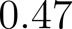; the bound 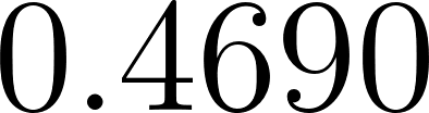is due to Shevtsova, 2011) and where . The error shrinks as , the same rate we saw in the Law of Large Numbers. Doubling improves the CLT approximation by a factor of 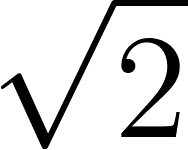, roughly .

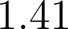The key qualitative message is that the approximation works better when:

• The original distribution is nearly symmetric (small third moment).
• The variance is well-behaved (not too small relative to the third moment).
• The sample size is large.

For heavy-tailed distributions or highly skewed distributions, the convergence can be quite slow, and much larger samples may be needed before the normal approximation is trustworthy.

The program demonstrates the CLT with a deliberately non-normal source: a distribution, which takes only the values and . This is about as far from a bell curve as you can get. We draw sample means of size 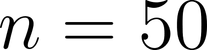and collect 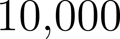of them:

The CLT predicts that these sample means should have:

• Mean
• Variance

The program computes both the theoretical predictions and the empirical values from the simulation, then prints a text histogram.

Look at that histogram. It is bell-shaped, even though the source distribution has only two possible values. The CLT has transformed a highly non-normal distribution into a nearly normal one, just by averaging 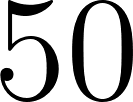independent draws.

The empirical mean (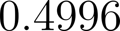) and variance (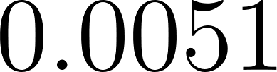) are very close to the CLT predictions of 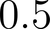and 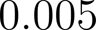. The small deviation in the mean is normal sampling variability. The program reseeds its random state on each run, so your exact numbers and bar heights will differ, but the bell shape and the match to the predictions are the same every time.

The CLT is the foundation for much of classical statistics. Confidence intervals, hypothesis tests (z-tests, t-tests), and regression analysis all rely on the normal approximation that the CLT provides.

Suppose we sample i.i.d. values with unknown mean and known standard deviation . By the CLT, the sample mean is approximately . A 95% confidence interval for is:

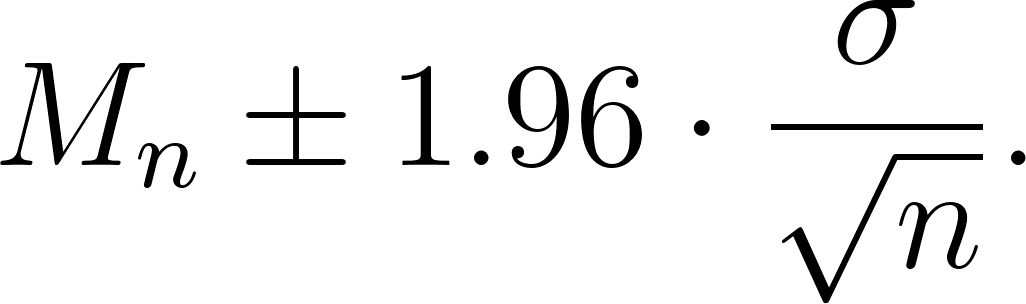
The number 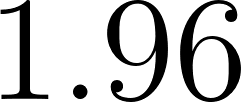is the 97.5th percentile of the standard normal (the two-sided critical value for 95% coverage). This interval is constructed so that in 95% of hypothetical repetitions of the experiment, the true mean would lie inside. The width of the interval shrinks as , the familiar Monte Carlo scaling.

When a pollster reports a “margin of error” of plus or minus 3%, that number comes from the CLT. The sample proportion is approximately normal (by the CLT), and the margin of error is about standard deviations of that normal distribution. For a sample of voters, the margin of error is approximately in percentage points, ignoring some multiplicative constants.

This is why pollsters usually collect around respondents. With , the margin of error is roughly 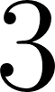percentage points. To halve it, they would need . To reach a margin of error of 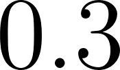percentage points, they would need , which is prohibitively expensive for most polls.

When a quality control engineer tests whether a manufacturing process is within spec, the CLT justifies using normal-based control charts even when the underlying process distribution is not normal. As long as the daily quantity being tracked is an average of many small independent effects, the CLT guarantees it will be approximately normal.

A common rule of thumb is that 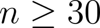is sufficient for the normal approximation to be reasonable. But this depends on the shape of the original distribution. For symmetric distributions, 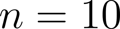or even 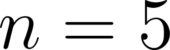may be enough. For highly skewed distributions, you may need or more.

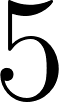
For situations, an alternative rule of thumb is that the normal approximation is good when both 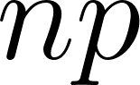and 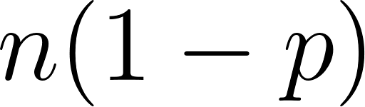exceed (some sources use ). This ensures that the distribution is far from being pushed against or and has enough room in both tails.

In our simulation, works beautifully for the symmetric case. If we used a instead, which is highly skewed, we would need a much larger to see the bell shape emerge.

When the CLT approximates a discrete distribution, such as a binomial count, a small adjustment sharpens the result. A discrete variable puts probability on the integers, while the approximating normal spreads probability continuously, so the event 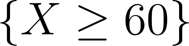is matched better by the normal event 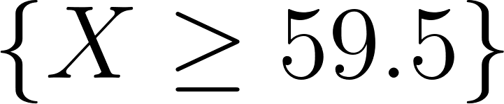: we widen each integer to the half-unit interval around it. To approximate 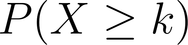for an integer-valued 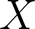, apply the normal approximation to ; to approximat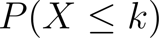e , use . This continuity correction typically cuts the approximation error several-fold for moderate , and it is worth applying whenever the underlying variable is a count. Problem 7.7 asks you to measure its effect against an exact binomial tail.

The CLT we have stated assumes i.i.d. random variables. Several extensions relax this:

• Lindeberg-Feller CLT: allows non-identically-distributed independent variables as long as no single term dominates in the variance.
• Martingale CLT: allows a specific kind of dependence (martingale differences), useful in stochastic processes.
• Multivariate CLT: extends to random vectors; the limit is a multivariate normal.
• Functional CLT (Donsker’s theorem): the entire path of a random walk converges to Brownian motion.

These extensions show how central the CLT is: even in complicated settings, sums of many small independent effects tend to look normal in some appropriate sense.

The Central Limit Theorem is the reason the normal distribution deserves its special status. It is not just one distribution among many. It is the attractor distribution for sums of independent random variables. Wherever independent effects accumulate, the normal distribution appears. This makes it the most important distribution in probability and statistics, and the CLT tells us why.

Problem 7.1. For the example simulation (), the CLT predicts is approximately . Compute the standard deviation of that normal (should be about 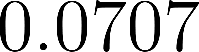) and identify the range 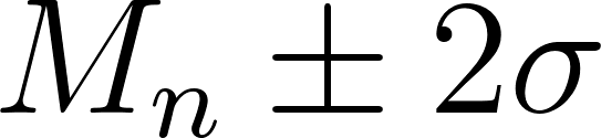. Approximately what fraction of the simulated sample means should fall inside this range?

Problem 7.2. Modify the simulation to use 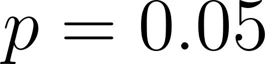(a highly skewed Bernoulli). With , is the histogram of sample means still bell-shaped? Increase to 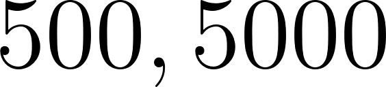. At what point does the bell shape become clear? Explain what you observe using the Berry-Esseen intuition.

Problem 7.3 (Uniform source). Replace the Bernoulli source with a source. Draw sample means with 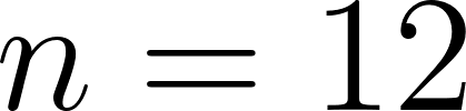. Confirm that the sample means look approximately . Because has mean 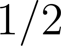and variance 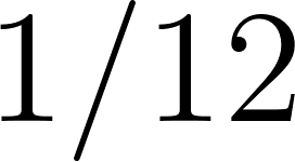, and the mean of 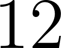samples has variance 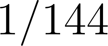, this is the CLT.

Problem 7.4 (Exponential source). Replace the source with an exponential of rate (mean , variance ). Draw sample means with , and 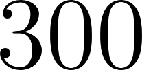. Because the exponential is right-skewed, the bell shape emerges more slowly than with the uniform. Compare the empirical histograms.

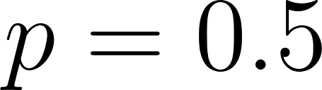
Problem 7.5 (Sample size for margin of error). How large a random sample do you need so that a 95% confidence interval for a Bernoulli proportion has half-width at most ? Use the worst case . What if the half-width must be ?

Problem 7.6 (CLT vs. Chebyshev). For a source with 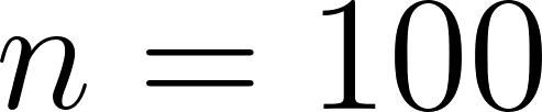, use Chebyshev’s inequality to bound . Then use the CLT to compute the same probability under the normal approximation. Compare the two bounds. Which is tighter?

Problem 7.7 (Approximating a binomial tail). Use the CLT (with continuity correction if you know it) to approximate 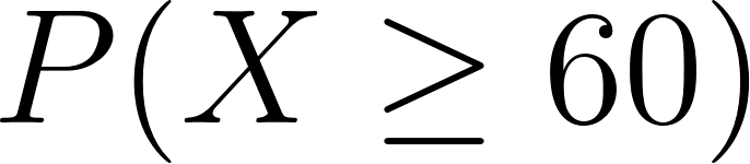where is . Then compute the exact binomial probability using the example program from Chapter 4. How close are the two answers?

Problem 7.8 (Coding exercise). Add a function that computes the empirical CDF of the sample means. Compare it against the CLT-predicted normal CDF and print the maximum absolute difference. This is a numerical estimate of the Berry-Esseen bound in action. Verify that this maximum difference shrinks as you increase .

Problem 7.9 (When the CLT fails). The CLT requires finite variance. Recall the Cauchy distribution from Chapter 6. Simulate sample means of Cauchy draws. Plot the histogram. Is it bell-shaped, or does it look like the Cauchy itself? Explain your observation.