Discrete Random Variables

So far we have been working with events as sets of outcomes. A random variable gives us a more convenient way to talk about randomness by assigning a number to each outcome. This lets us work with averages, spreads, and distributions instead of individual events.

The example program for this chapter is in the file 03_discrete_random_variables.lisp.

Working with events directly gets cumbersome once questions become quantitative. Consider rolling two dice and asking about the sum. We could describe the events “sum equals 2,” “sum equals 3,” …, “sum equals 12” one at a time and compute their probabilities separately. But it is much cleaner to introduce a single object, the sum-of-dice random variable, and treat all these events as questions about it.

Random variables give us the language for summary statistics like mean and variance, for comparing distributions, for talking about correlations between quantities, and for stating limit theorems. They are the mathematical objects that a probability calculation is usually really about.

A random variable 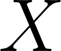is a function from the sample space to the real numbers. It assigns a numerical value to each outcome. For example, if we roll two dice, we can define to be the sum of the two dice. Then maps the outcome 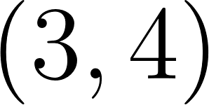to the value 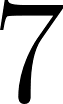, the outcome 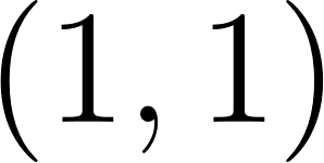to the value , and so on.

The name “random variable” is slightly misleading. A random variable is not itself random; it is a deterministic function. The randomness comes from the underlying experiment. Once the outcome 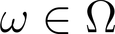is fixed, 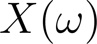is a definite number. This distinction matters when we discuss expectation and variance: those are properties of the function together with the probability measure 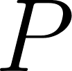, not of any particular value.

The support of a random variable is the set of values it can actually take. For the sum of two dice, the support is . For a coin flip encoded as or , the support is 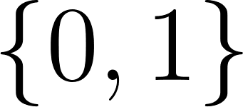. A discrete random variable takes values in a countable set, often a finite set of integers.

A technical requirement hides behind the word “function.” For 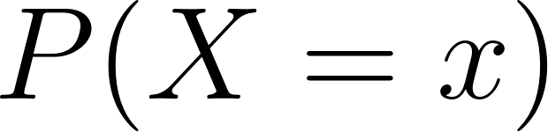and 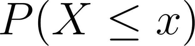to make sense, the sets and must be events, that is, members of the -algebra 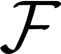from the previous chapter. A function with this property is called measurable, and only measurable functions qualify as random variables. In the discrete case, where is the full power set, every function is measurable and the requirement is automatic, so we will not raise it again until continuous distributions make it matter.

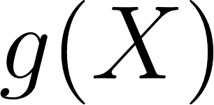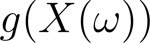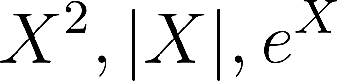Any function of a random variable is again a random variable. If is a random variable and is a function, then assigns to each outcome . So , and are all random variables built from .

The simplest and most useful random variable is the indicator of an event. Given an event 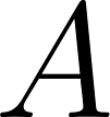, its indicator 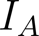is defined as:

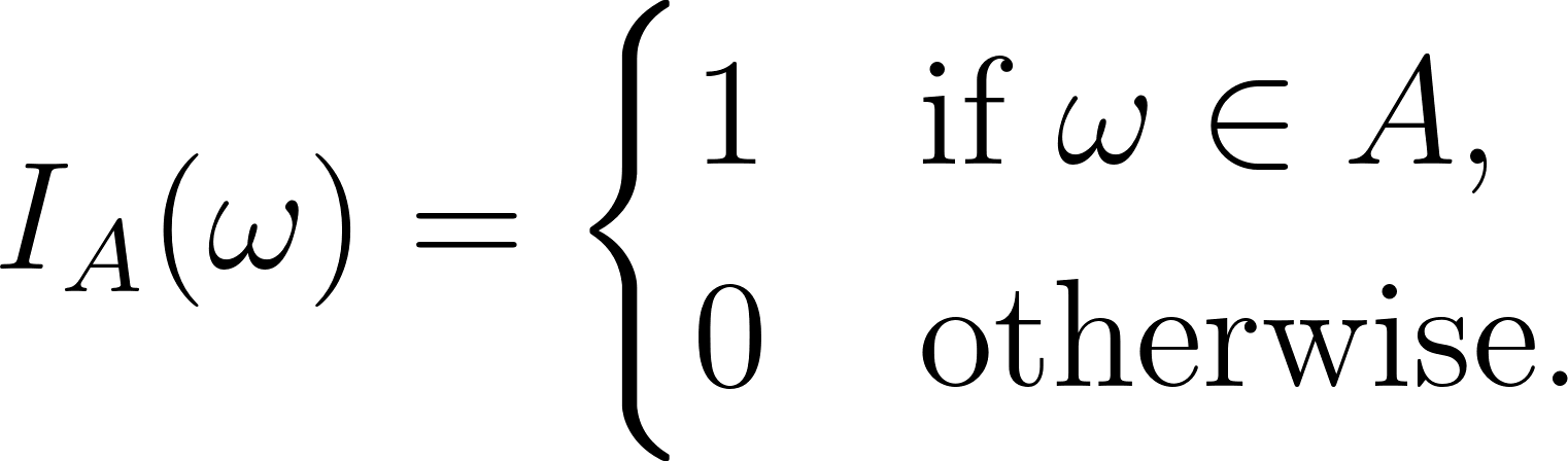
Indicator random variables are the bridge between events and expectations. Note that . Every probability can be written as an expectation of an indicator. This turns out to be extraordinarily useful when combined with linearity of expectation, as we will see below.

The probability mass function (PMF) of a discrete random variable gives the probability that equals a specific value :

The PMF satisfies two properties: every value 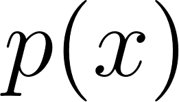is non-negative, and the sum of all values equals . These are the discrete analogues of the Kolmogorov axioms.

In the example program, we represent a PMF as an alist mapping values to probabilities:

1 (defstruct pmf
2   "A discrete probability mass function represented as an alist
3    mapping value -> probability."
4   table)

The function pmf-total-probability verifies the normalization axiom by summing all the probabilities. For a valid PMF, this sum must equal 1.

The cumulative distribution function (CDF) accumulates probability up to a given value:

The CDF is a non-decreasing function: as increases, 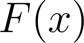can only go up or stay the same. It starts at (for values below the smallest possible outcome) and ends at (for values above the largest possible outcome). For discrete random variables, the CDF is a step function that jumps at each value in the support of by an amount equal to .

The CDF is more universal than the PMF: it is defined for any real-valued random variable, discrete or continuous. Two random variables that share the same CDF share the same distribution. When we talk about “the distribution of X$,” the CDF is the most general representation.

1 (defun cdf (p x)
2   "Cumulative distribution function F_X(x) = P(X <= x)."
3   (reduce #'+ (mapcar (lambda (entry)
4                         (if (<= (car entry) x) (cdr entry) 0))
5                       (pmf-table p))))

The expected value (or mean) of a random variable is the probability-weighted average of all its possible values:

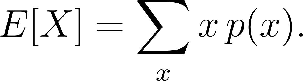
The expected value represents the long-run average if we repeated the experiment many times. If we rolled two dice a million times and averaged all the sums, we would get a number very close to .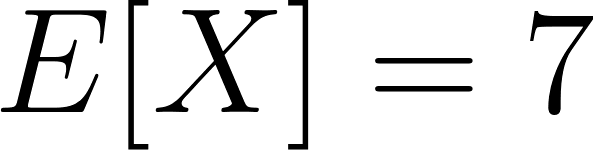

1 (defun expectation (p)
2   "E[X] = sum of x * p_X(x), the mean of the distribution."
3   (reduce #'+ (mapcar (lambda (entry) (* (car entry) (cdr entry)))
4                       (pmf-table p))))

More generally, for any function of a random variable , the law of the unconscious statistician says:

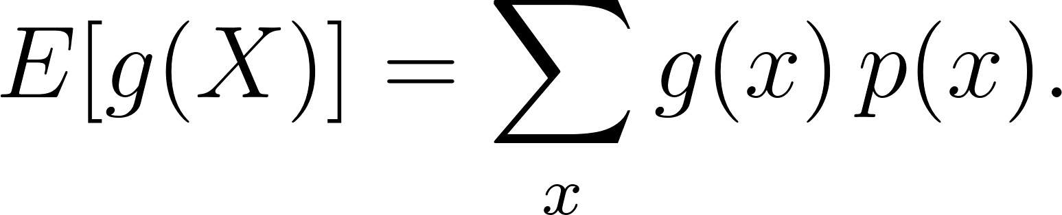
This lets us compute the expected value of any function of without needing to derive the distribution of first.

A key property of expectation is linearity. For any constants and :

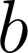And for any two random variables and 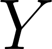, even if they are dependent:

Linearity of expectation is one of the most useful tools in probability. It lets us compute the expected value of a sum without knowing anything about the relationship between the variables. This holds even if and are strongly correlated, which is often surprising to newcomers.

One striking application uses indicator random variables. Suppose we want the expected number of pairs among coin flips that both show heads. Let 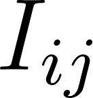be the indicator that flips 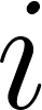and 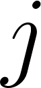both show heads. The count of matching heads pairs is 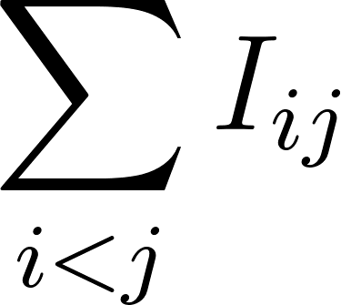. By linearity, the expected count is 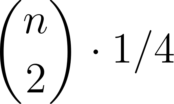, regardless of whether we treat the flips as independent or not. Indicator variables plus linearity turn many counting-in-expectation problems into one-line calculations.

The variance measures how spread out a distribution is around its mean:

There is a computational shortcut that is often easier to use:

This identity comes from expanding 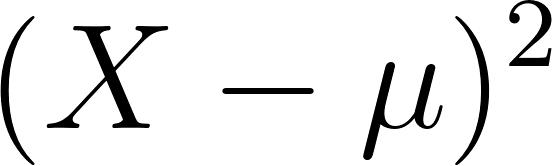and using linearity of expectation. The program uses this shortcut:

1 (defun variance (p)
2   "Var(X) = E[X^2] - (E[X])^2."
3   (let ((ex (expectation p)))
4     (- (expectation-of-square p) (* ex ex))))

The standard deviation is the square root of the variance. It has the same units as the random variable itself, which makes it more interpretable. A standard deviation of 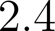for the sum of two dice means that a typical roll deviates from the mean of by about points.

Unlike expectation, variance is not linear in general. For a constant :

For a sum of two random variables:

where is the covariance. When and are independent, the covariance is zero and . This additivity of variance for independent variables is one of the reasons independence is so useful.

The covariance carries the product of the units of and , which makes its numerical value hard to interpret on its own. Dividing by the two standard deviations strips the units and yields the correlation coefficient:

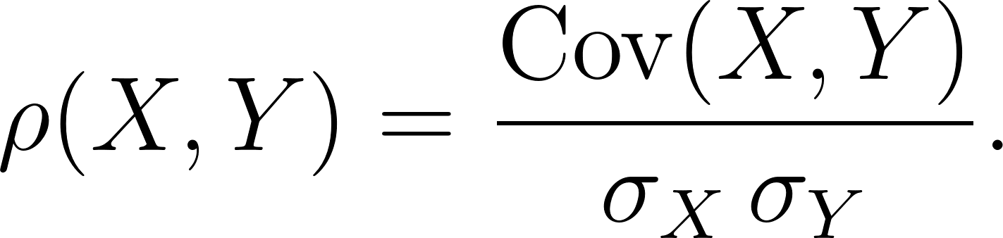
The Cauchy-Schwarz inequality forces , with 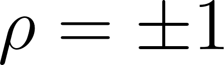exactly when is an affine function of . A correlation of means and are uncorrelated. Independence implies zero correlation, but the converse fails: uncorrelated variables can still be dependent, because detects only linear association.

For a sum of many variables the two-term rule generalizes to

When the variables are pairwise uncorrelated, every cross term drops out and the variance of the sum is just the sum of the variances. This is the fact that makes the variance of a sample mean shrink like 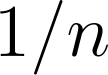, the engine of the Law of Large Numbers two chapters from now.

Given a random variable with mean and standard deviation , its standardized form is:

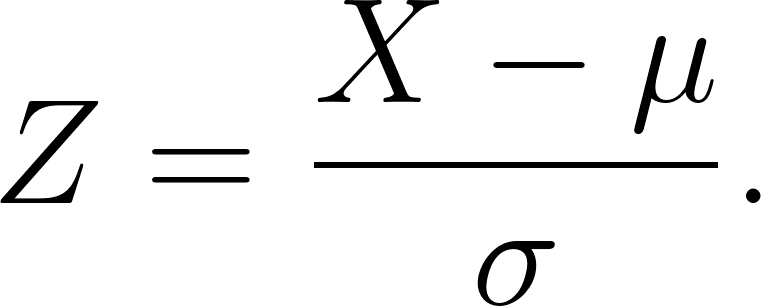
By construction, 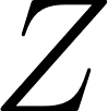has mean and variance . Standardization lets us compare distributions on a common scale and is essential for stating limit theorems like the Central Limit Theorem in a clean form.

The mean and variance are the first two members of a larger family. The 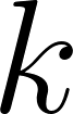-th moment of is 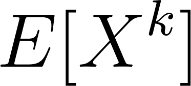, and the -th central moment is 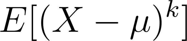. The mean is the first moment; the variance is the second central moment. The third and fourth central moments, once standardized, describe the shape of a distribution beyond its location and spread:

Skewness measures asymmetry: a positive value signals a long right tail. Kurtosis measures how heavy the tails are relative to a normal distribution, whose kurtosis is .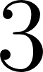

All of these moments are packaged together by the moment generating function (MGF):

defined for those where the sum is finite. The name comes from a small miracle: differentiating 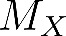at 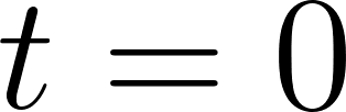reproduces the moments one at a time,

This follows from expanding 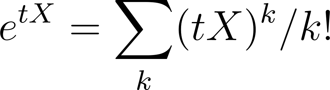and taking the expectation term by term. The MGF has two properties that make it a workhorse of the later chapters. First, it turns sums of independent variables into products: if and are independent then , because the expectation of a product of independent quantities factors. Second, it determines the distribution uniquely: two random variables with the same MGF on an interval around have the same distribution. Together these facts let us identify the distribution of a sum by multiplying MGFs, and they underlie one standard proof of the Central Limit Theorem. A close relative, the characteristic function , exists for every distribution even when the MGF does not, and is the tool of choice in the rigorous theory.

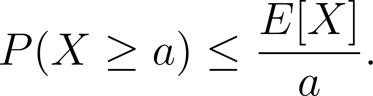
Given only the mean and variance of a random variable, we can already bound how much probability can lie far from the mean. Two classic bounds appear again and again.

Markov’s inequality: for a non-negative random variable and any :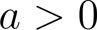

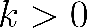
Chebyshev’s inequality: for any random variable with mean and finite variance 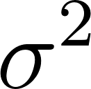and any :

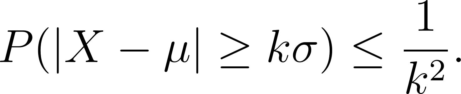
Chebyshev’s inequality follows from Markov’s inequality applied to the non-negative random variable . It says that the probability of being more than standard deviations from the mean is at most 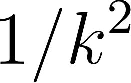, no matter what the distribution is. This is the key ingredient in the proof of the Weak Law of Large Numbers, which we will meet in a later chapter.

These inequalities are usually quite loose: for a specific distribution you can often do much better. But their power is that they work for every distribution with finite mean or variance.

The program demonstrates three distributions. The first is a loaded die where the probability of rolling a 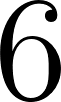is 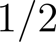and the remaining probabilities are 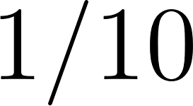each. The mean is 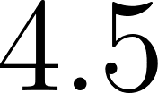(higher than the fair die’s 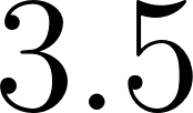) because the loaded die favors high values.

The second is a Bernoulli distribution with 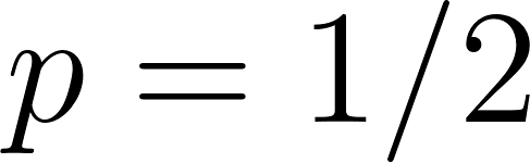. A Bernoulli random variable takes only two values: (success) with probability , and (failure) with probability 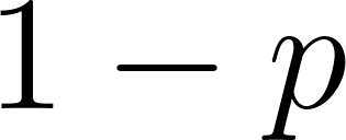. Its mean is and its variance is 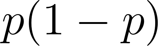. The Bernoulli distribution is the simplest discrete distribution and the building block for the binomial distribution we will study in the next chapter.

The third is the sum of two fair dice. This is the classic triangular distribution: the probability of rolling a is highest (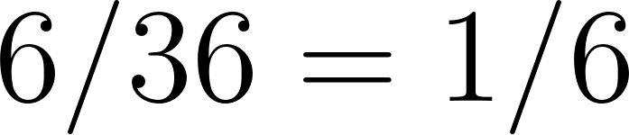) because there are more ways to make than any other sum, while the probability of rolling a or 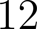is lowest ( 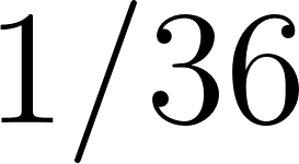each) because there is only one way to make each.

The program does more than tabulate PMFs. It also demonstrates four ideas from earlier in this chapter, each in a few lines.

Convolution. The PMF of a sum of independent variables is the convolution of their PMFs, . The function convolve-pmfs rebuilds the two-dice distribution from two single dice, and its mean () and variance (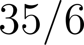) match the direct computation. This is the coding exercise from Problem 3.8.

Standardization. standardize maps each value to 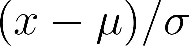, producing the PMF of . The program confirms that has mean and variance , as Problem 3.7 asks.

Chebyshev’s inequality. For the dice sum the program prints the actual next to the distribution-free bound , showing the bound holds, and is loose, at every .

Covariance and correlation. Using a joint PMF over value pairs, the program computes 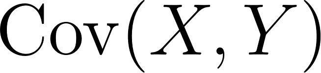and 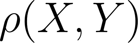for two independent dice (both ) and for a single die paired with the two-dice sum, where the covariance is and the correlation is .

 1 === Loaded Die ===
 2 Distribution of LoadedDie:
 3   Normalization check Σ p(x) = 1
 4   x=1 : P(X=x)=1/10  P(X<=x)=1/10
 5   x=2 : P(X=x)=1/10  P(X<=x)=1/5
 6   ...
 7   x=6 : P(X=x)=1/2  P(X<=x)=1
 8   E[LoadedDie]   = 9/2 =  4.5
 9   Var(LoadedDie) = 13/4 = 3.25
10   sigma   =  1.8
11 
12 === Sum of Two Fair Dice ===
13   E[DiceSum]   = 7 =  7.0
14   Var(DiceSum) = 35/6 = 5.83
15   sigma   = 2.42
16 
17 === Convolution: single die + single die ===
18   E[die+die]   = 7 =  7.0 (matches DiceSum mean 7)
19   Var(die+die) = 35/6 = 5.83 (matches DiceSum var 35/6)
20 
21 === Standardization: Z = (X - mu)/sigma ===
22   mean(Z) =  0.000 (should be 0)
23   var(Z)  =  1.000 (should be 1)
24 
25 === Chebyshev's Inequality (dice sum) ===
26   k     actual P(|X-mu|>=k sigma)   bound 1/k^2
27   1.0               0.3333            1.0000
28   1.5               0.1667            0.4444
29   2.0               0.0556            0.2500
30   2.5               0.0000            0.1600
31 
32 === Covariance and Correlation ===
33   Two independent dice (X, Y):
34     Cov =  0.000  rho =  0.000 (independent => 0)
35   A die and the two-dice sum (X, X+Y):
36     Cov =  2.917  rho =  0.707 (rho = 1/sqrt(2) ~ 0.707)

The normalization check confirms that the PMF sums to . The expected value of the dice sum is exactly , and the variance is , which is about 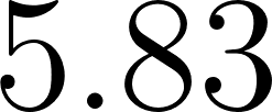. These exact rational results come from Lisp’s built-in rational arithmetic.

Notice that the mean of the sum of two dice is , which equals 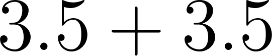, the sum of the means. This is linearity of expectation in action. The variance is , which equals , the sum of the variances of each fair die (since the two rolls are independent). This is the additivity of variance for independent random variables.

Expected value and variance are the two most important summary statistics for any random variable. Throughout the rest of this book, we will compute means and variances for every distribution we encounter. The formulas 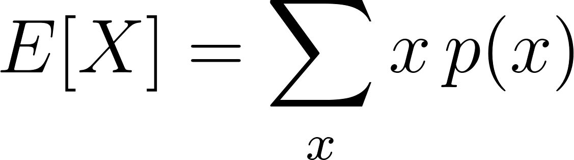and are tools you will use again and again. Linearity of expectation and Chebyshev’s inequality will show up in the proofs of the Law of Large Numbers and the Central Limit Theorem in later chapters.

Problem 3.1. Compute 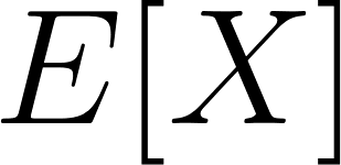and 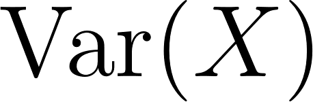for a fair six-sided die directly from the definition. Confirm your answer against the program’s output for the sum of two dice (using linearity of expectation and additivity of variance for independent variables).

Problem 3.2. For the loaded die in the example (, all other faces ), what is 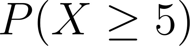? What is 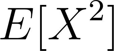? Verify the variance formula using your computed values.

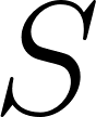
Problem 3.3 (Linearity of expectation). Consider rolling three fair dice. Let 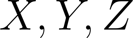be the three roll values, and let . Use linearity of expectation to compute 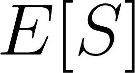. Now use additivity of variance for independent variables to compute 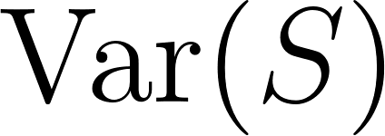. Verify your answers by extending the example program to enumerate the 216-outcome sample space and directly compute the mean and variance of .

Problem 3.4 (Indicator random variables). A word is chosen uniformly at random from a 26-letter alphabet, one letter at a time, for a word of length . Let be the number of vowels in the word (a, e, i, o, u count as vowels). Using indicator random variables and linearity of expectation, compute for a word of length .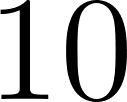

Problem 3.5 (Chebyshev’s inequality). For a distribution with mean 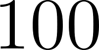and standard deviation , use Chebyshev’s inequality to bound the probability that lies outside the interval 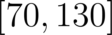. Then use the same inequality to bound the probability that lies outside 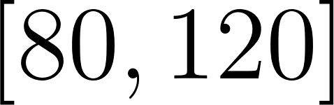. Comment on how the bound tightens as the interval widens.

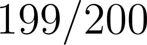
Problem 3.6 (Comparing distributions). A game offers two prizes: Game A pays dollar with probability and pays dollars with probability . Game B pays dollars with probability 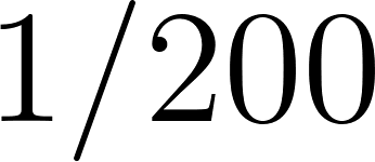and pays dollars with probability . Compute the mean and variance for each game. Which game has the same expected payout? Which has more variance? Which would you rather play if you could play it just once? If you could play it a million times?

Problem 3.7 (Coding exercise). Extend the PMF library with a function standardize that takes a PMF for and returns a PMF for . Verify numerically that the new PMF has mean and variance .

Problem 3.8 (Sum of two independent PMFs). Add a function convolve-pmfs to the example program that takes two PMFs (representing independent random variables and ) and returns the PMF of the sum 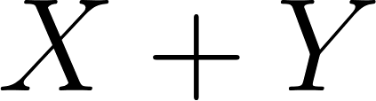. Use it to construct the PMF of the sum of two fair dice starting from the PMF of a single die. Confirm that the resulting mean and variance match the direct computation.