Binomial and Geometric Distributions

Two of the most important discrete distributions arise from repeating the same simple experiment over and over. If we flip a biased coin repeatedly, we can ask two natural questions: how many successes happen in a fixed number of flips, and how long do we wait for the first success? These questions lead to the binomial and geometric distributions.

The example program for this chapter is in the file 04_binomial_geometric.lisp.

Bernoulli Trials

A Bernoulli trial is the simplest random experiment with two outcomes: “success” (with probability Code Test ) and “failure” (with probability 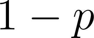). If we let 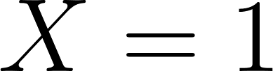on success and 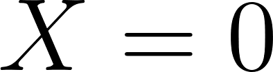on failure, then 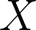has the 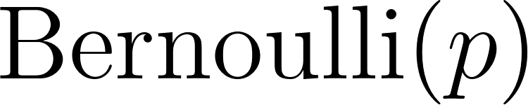distribution with:

The Bernoulli trial is the atom from which we build more complex distributions. The Bernoulli distribution itself is named after Jakob Bernoulli, the seventeenth-century Swiss mathematician whose posthumous Ars Conjectandi (1713) contains the first published proof of what we would now call the Weak Law of Large Numbers for Bernoulli trials.

A key modeling question is when a Bernoulli trial is a reasonable idealization of reality. It works well for a coin flip or a fair random selection, but many real situations only approximate the assumptions of a Bernoulli trial. Two trials are only truly “the same” if the mechanism that produces them is unchanged and the outcome of one does not influence the other. Whenever we build a binomial or geometric model, we are implicitly making these assumptions.

The Binomial Distribution

If we run Code Test independent trials and count the number of successes, the count has the binomial distribution, written . The probability of getting exactly 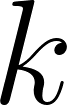successes is:

where 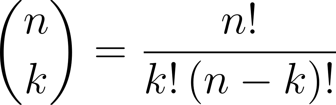Code Test is the binomial coefficient, the number of ways to choose which of the trials are the successes. The factor 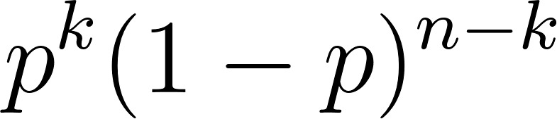is the probability of any one specific sequence with successes and 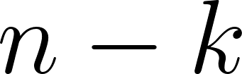failures, and 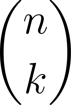counts how many such sequences there are.

Two ingredients are worth pausing over. First, the factor Code Test arises because the trials are independent: the joint probability of a specific sequence of outcomes is the product of the individual probabilities. If the trials were correlated, this factorization would fail. Second, the binomial coefficient is exactly the number of arrangements of the successes among the Code Test positions. Multiplying gives us the total probability of the event “exactly k$ successes.”

The program computes binomial coefficients iteratively to avoid huge intermediate factorials:

1 (defun binomial-coefficient (n k)
2   "C(n,k) = n!/(k!(n-k)!). Computed iteratively to avoid huge
3    intermediate factorials."
4   (if (or (< k 0) (> k n))
5       0
6       (loop with result = 1
7             for i from 1 to k
8             do (setf result (* result (/ (+ n (- k) i) i)))
9             finally (return (round result)))))

The mean and variance of the binomial distribution are:

The mean formula has an intuitive explanation via linearity of expectation. Each trial contributes Code Test to the expected count on average, and there are independent trials, so the expected total is 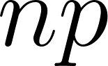. Similarly, since the trials are independent, the variance of the count is the sum of the variances of the individual Bernoulli indicators, which is .

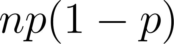The Binomial as a Sum of Bernoullis

Formally, if Code Test are i.i.d. random variables and , then 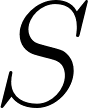has the distribution. This decomposition is often the fastest way to prove properties of the binomial: linearity of expectation gives 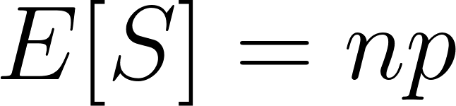in one line, and independence gives in another. Any theorem you know about sums of independent random variables applies immediately to binomial random variables.

The same decomposition hands us the moment generating function for free. A single Code Test variable has MGF , and because the trials are independent the MGF of their sum is the product of the individual MGFs:

Reading the mean and variance off the first two derivatives at 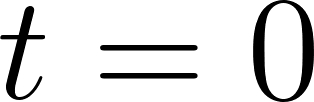Code Test recovers and yet again. The product form also proves a reproductive property: if and are independent with the same , then , since their MGFs multiply to . The trial picture makes this obvious too: pooling 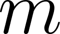trials with more of the same kind simply gives 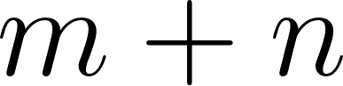trials.

The Normal Approximation

For large Code Test , the binomial distribution is closely approximated by a normal distribution with mean and variance . This follows from the Central Limit Theorem (Chapter 7). A useful rule of thumb is that the normal approximation is reasonable when both and 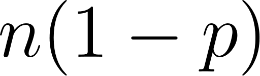are at least 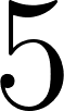. For a single coin flip (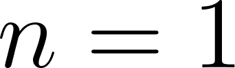), the binomial is nowhere near normal; for Code Test flips, the normal is nearly indistinguishable from the exact binomial.

The Poisson Limit

There is a beautiful limit that connects the binomial distribution to another famous distribution. Suppose Code Test grows large and shrinks such that the product 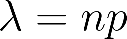is held constant. Then the binomial distribution converges to the Poisson distribution with parameter :

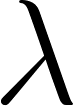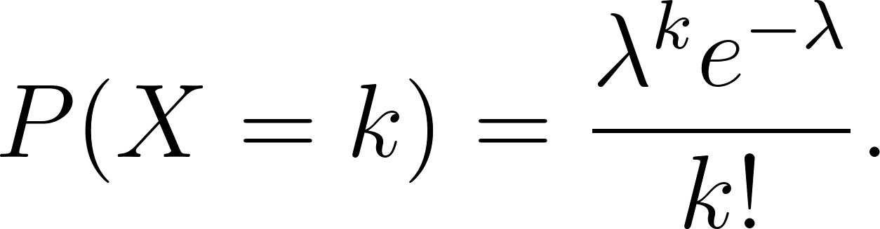
This is why Poisson distributions describe rare events counted over long stretches: the number of decays of a radioactive sample in one second, the number of typos on a page, the number of calls arriving at a call center in a minute. Each event is one of a huge number of possibilities, each with tiny individual probability; the total count is nearly Poisson.

The program makes this concrete. It tabulates Code Test , , and 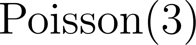side by side (all with mean 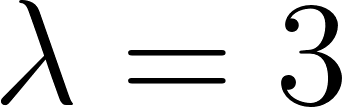), and the binomial columns march toward the Poisson one as grows. It also reports the mode of , the most likely count, from the closed form 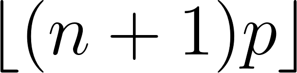(Problem 4.9).

The Geometric Distribution

The geometric distribution answers a different question: if we run Code Test trials until the first success occurs, how many trials do we need? If 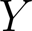is the number of trials (including the successful one), then:

This formula reads as “k - 1$ failures followed by one success.” The geometric distribution is a valid PMF because it sums to a geometric series: Code Test .

A note on conventions: some books define Code Test as the number of failures before the first success, so takes values 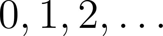rather than 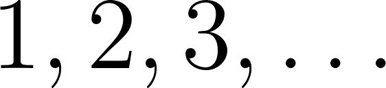. The formulas are almost identical but the mean shifts by . Always check which convention a book or library uses.

The mean and variance are:

The mean 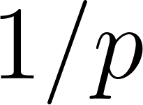Code Test makes intuitive sense. If the success probability is 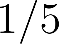, you wait about trials on average. The smaller the success probability, the longer you expect to wait. The variance grows as shrinks, so waiting times for rare events are both long and highly variable.

Why the Mean Is 1/p

The formula 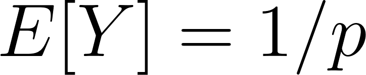Code Test has a derivation that uses no series at all, only the structure of the experiment. Condition on the first trial. With probability it succeeds and 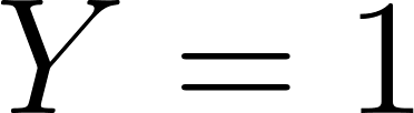. With probability it fails, one trial is spent, and the remaining wait is a fresh, statistically identical copy of . Hence

Solving for 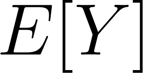Code Test gives . The same conditioning trick applied to 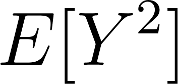produces the variance 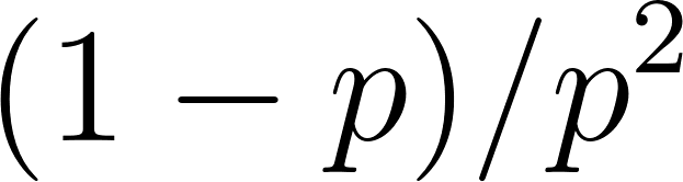without summing a single geometric series. This self-consistency argument, in which a quantity is expressed in terms of itself one step later, is the discrete seed of the first-step analysis we will use for Markov chains in the final chapter.

The tail probability 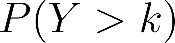Code Test has an especially clean form:

This says: the probability that we still have not had a success after Code Test trials is the probability that all trials failed, which is 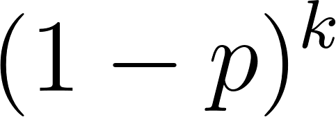by independence. We will use this formula in the proof of the memoryless property below.

The Memoryless Property

The geometric distribution has a remarkable property called memorylessness. It says that the past does not affect the future. Specifically:

If you have already waited Code Test trials without a success, the probability of waiting at least more trials is the same as if you had just started. The distribution “forgets” how long you have been waiting.

The program demonstrates this property directly:

1 (defun demonstrate-memoryless-property (p m n)
2   "Show P(Y > m+n | Y > m) = P(Y > n) for a geometric random variable Y."
3   (let ((conditional (/ (geometric-tail p (+ m n)) (geometric-tail p m))))
4     (format t "  Memoryless property check (p=~a, m=~a, n=~a):~%" p m n)
5     (format t "    P(Y > m+n | Y > m) = ~a = ~4f~%" conditional (float conditional))
6     (format t "    P(Y > n)          = ~a = ~4f~%" (geometric-tail p n)
7             (float (geometric-tail p n)))))

The proof is a one-liner. Since Code Test , we have:

The geometric is the only discrete distribution on 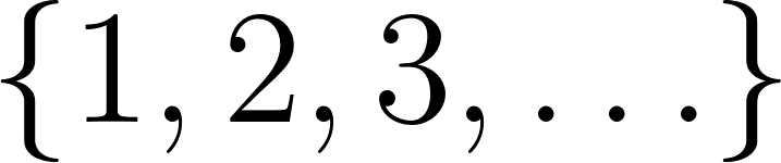Code Test with this property. In the continuous world, its analogue is the exponential distribution, which we will meet in the next chapter.

Other Distributions from Bernoulli Trials

The binomial and geometric are two members of a small family of distributions built from Bernoulli trials. Two others are worth naming, even briefly.

The negative binomial distribution generalizes the geometric: instead of waiting for the first success, we wait for the Code Test -th success. The number of failures before the -th success has a negative binomial distribution. The geometric distribution is the special case .

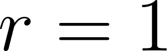The hypergeometric distribution replaces sampling with replacement (where each trial is truly independent) with sampling without replacement from a finite population. If we draw n cards from a shuffled deck without replacement and count how many are aces, the count is hypergeometric, not binomial, because each draw changes the composition of the remaining deck. When the population is much larger than the sample, the hypergeometric distribution is well approximated by the binomial.

Real-World Applications

The binomial distribution is the workhorse of any situation involving repeated trials with a fixed success probability. It underlies:

Opinion polling: the number of respondents in a random sample who support a candidate.
Quality control: the number of defective items in a batch.
A/B testing: the number of users in a test group who click a button.
Genetics: the number of offspring with a particular trait, under simple Mendelian assumptions.

The geometric distribution is the workhorse of any situation involving waiting for a first success:

Sales: the number of sales calls until the first sale.
Networking: the number of packet transmissions until a successful acknowledgment.
Reliability: the number of trials until a machine failure, if the failure probability is constant per trial.
Games: the number of rolls until you get a specific number on a die.

The memoryless property is a strong assumption in these applications. It is only true if the underlying success probability really is constant across trials. In many real settings the true success probability changes over time, and the geometric distribution is only a first approximation.

Running the Example

 1 === Binomial Distribution: n=10, p=0.3 ===
 2   E[X] = n p = 3,  Var(X) = n p (1-p) = 21/10
 3   P(X=0) = 0.0282   CDF F(0) = 0.0282
 4   P(X=1) = 0.1211   CDF F(1) = 0.1493
 5   P(X=2) = 0.2335   CDF F(2) = 0.3828
 6   P(X=3) = 0.2668   CDF F(3) = 0.6496
 7   ...
 8   P(X=10) = 0.0000   CDF F(10) = 1.0000
 9 
10 === Geometric Distribution: p=0.2 ===
11   E[Y] = 1/p = 5,  Var(Y) = (1-p)/p^2 = 20
12   P(Y=1) = 1/5 =  0.2   P(Y>1) = 4/5 =  0.8
13   P(Y=2) = 4/25 = 0.16   P(Y>2) = 16/25 = 0.64
14   ...
15 
16 === Memoryless Property ===
17   Memoryless property check (p=1/5, m=3, n=2):
18     P(Y > m+n | Y > m) = 16/25 = 0.64
19     P(Y > n)          = 16/25 = 0.64
20 
21 === Poisson Limit of the Binomial (lambda = n p = 3) ===
22   As n grows with n p = 3 fixed, Binomial(n, 3/n) -> Poisson(3).
23    k   Binom(50,0.06)   Binom(500,0.006)   Poisson(3)
24   0         0.04533          0.04934         0.04979
25   1         0.14467          0.14891         0.14936
26   2         0.22624          0.22427         0.22404
27   3         0.23106          0.22472         0.22404
28   4         0.17329          0.16854         0.16803
29   5         0.10176          0.10092         0.10082
30   6         0.04872          0.05026         0.05041
31 
32 === Binomial Mode ===
33   Most likely k for Binomial(10, 0.3) = 3 (the peak of the PMF above)

The binomial distribution with 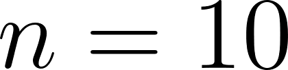Code Test and 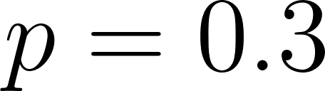is peaked around 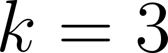(the mean), with the probability declining on both sides. The CDF rises from near to exactly , confirming that the PMF sums to .

The geometric distribution with 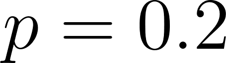Code Test is monotonically decreasing: the most likely outcome is (a success on the very first trial) with probability 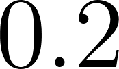, and longer waits become progressively less likely.

The memoryless property check confirms that Code Te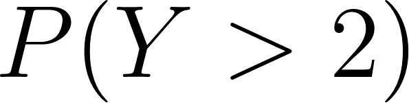st equals , both being . The past waiting time of 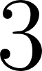trials has no effect on the future.

Why This Matters

The binomial distribution appears whenever we count successes in repeated independent trials: opinion polling, quality control, A/B testing, and many other applications. The geometric distribution models waiting times: how many calls until a sale, how many attempts until a success, how many packets until a collision. Together, these two distributions cover a huge range of practical discrete probability problems.

Problem Set

Problem 4.1. A fair coin is flipped Code Test times. Using the binomial PMF from the example program, compute the probability of getting exactly heads, at least 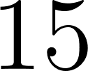heads, and at most heads. Then verify that the probabilities of “exactly k$ heads” for sum to .

Problem 4.2. A political poll interviews Code Test randomly chosen voters. Suppose the true fraction supporting a candidate is 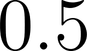. Using the binomial distribution, what is the probability that the observed proportion in the poll lies within one percentage point of (that is, between 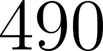and 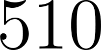supporters)? You will probably want to use the normal approximation for this one; check your answer with the exact binomial as well.

Problem 4.3 (Comparing means and variances). Compute the mean and variance of Code Test and of . Which has the larger variance? Explain in words why symmetry (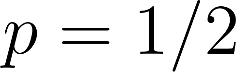) maximizes the variance among all distributions.

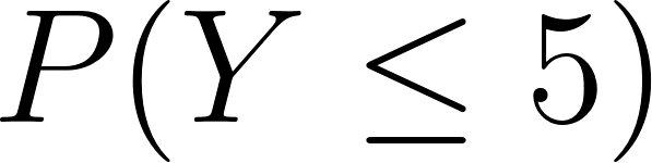
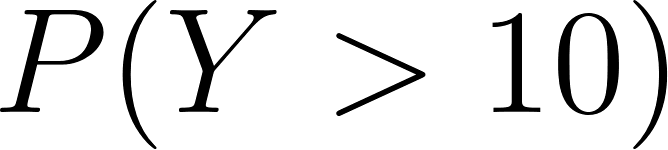
Problem 4.4 (Geometric waiting). A die is rolled repeatedly. Let Code Test be the number of rolls until the first 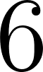appears. What is ? What is ? What is ? Now compute and confirm it equals 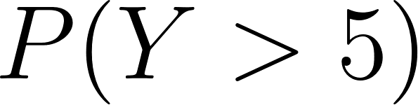, the memoryless property.

Problem 4.5 (Memorylessness and gambler’s fallacy). A slot machine hits a jackpot with probability Code Test on each pull, independently of past pulls. A gambler has just experienced losing pulls in a row and reasons that a jackpot must be “due” soon. Use the memoryless property to explain why this reasoning is wrong. What does the memoryless property say about the distribution of remaining pulls until the next jackpot?

Problem 4.6 (Simulation vs. theory). Extend the example program to simulate 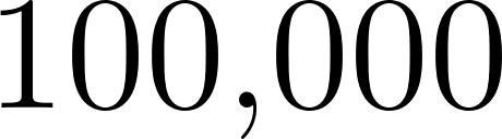Code Test trials of . Compare the empirical PMF against the theoretical PMF. Also compute the empirical mean and variance and compare against and .

Problem 4.7 (Poisson approximation). Compute the exact Code Test probability that 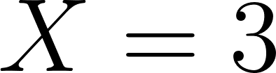. Then compute the Poisson approximation with , using . Compare the two values. The Poisson formula uses no factorial-of- and is much cheaper to compute.

Problem 4.8 (Waiting for multiple successes). In a game where each trial succeeds with probability Code Test , what is the expected number of trials needed to accumulate successes? Hint: by linearity of expectation, this is the sum of independent geometric waiting times. Use this to compute the answer directly.

Problem 4.9 (Coding exercise). Write a function binomial-mode that, given Code Test and , returns the value of that maximizes the binomial PMF. There is a closed-form expression involving 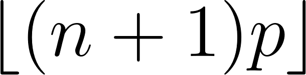. Verify your function against a direct search for a few values of and .

Up next

Continuous Distributions