Continuous Distributions
When a random variable can take any value in an interval, we call it a continuous random variable. The height of a randomly chosen person, the time until a radioactive decay, and the noise in an electrical signal are all continuous. Because a continuous variable can take uncountably many values, the probability of any single exact value is zero. We need a new tool: the probability density function.
The example program for this chapter is in the file 05_continuous_distributions.lisp.
Why Continuous Random Variables?
The step from discrete to continuous random variables is more than a technical convenience. Many quantities we care about are, at least in the model we use for them, genuinely continuous. Time, position, temperature, angle, mass, and voltage are all naturally described by real numbers, and no discrete PMF can capture their full range in a clean way.
There is a philosophical subtlety here. In the physical world, everything we measure is finite-resolution, so strictly speaking we could always model measurements as taking finitely many values. But the mathematics of continuous distributions is often much simpler than the mathematics of a very fine-grained discrete grid. Calculus tools such as differentiation, integration, and change of variable apply naturally to continuous distributions. So we treat continuous models as an idealization that trades a small amount of realism for a large gain in mathematical tractability.
From Probability Mass to Probability Density
For a discrete random variable, the PMF gives 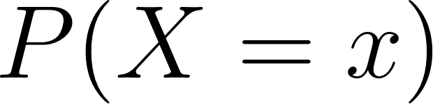 directly. For a continuous random variable,
  for every single point
  . Instead, we use the probability density function (PDF)
 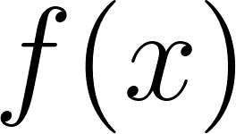 . Probability is now the area under the density curve:
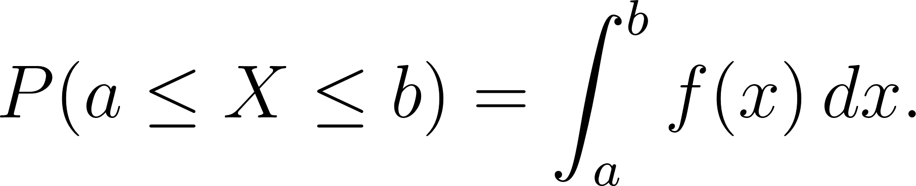
A valid PDF satisfies two conditions: 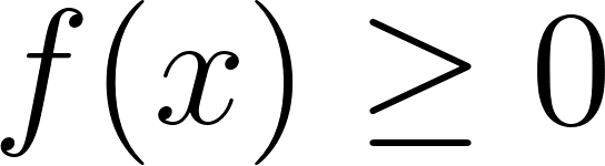 everywhere, and
 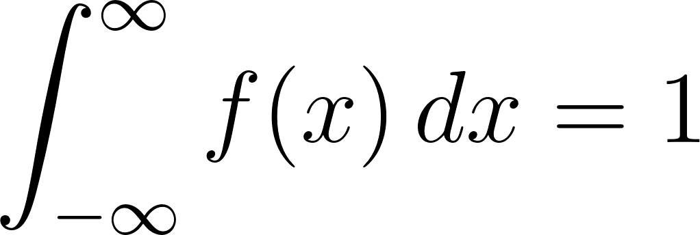 . The PDF itself is not a probability and can exceed
  . Only the integral over an interval is a probability.
This last point is worth emphasizing. If I tell you that the PDF of a certain distribution at 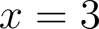 is
is 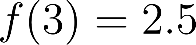 , that number does not mean the probability of
 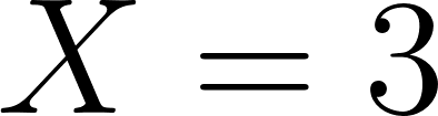 . It means that the density of probability is
 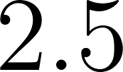 per unit length near . To get a probability, you integrate over an interval; to compare two densities you compare the ratio of densities in the same neighborhood.
The cumulative distribution function works the same way as in the discrete case:  . The relationship between the PDF and CDF is that the PDF is the derivative of the CDF.
Formally, the CDF 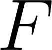 is what really characterizes the distribution. The PDF is defined (when it exists) as the derivative of the CDF. Not every random variable has a PDF, but every real-valued random variable has a CDF.
A random variable that has a density is called absolutely continuous, and the density is the derivative of the CDF wherever that derivative exists. Not every continuous CDF comes from a density: there are exotic singular distributions whose CDF rises continuously yet has zero derivative almost everywhere. There are also mixed distributions that place point masses at some values and spread density over others, such as a waiting time that equals exactly  with positive probability and is otherwise continuous. The CDF handles all of these uniformly, which is the deeper reason it, not the PDF, is taken as the defining object of a distribution. Every continuous example in this book is absolutely continuous, so a density always exists.
The Quantile Function
Sometimes we want the inverse question: given a probability, what value of 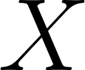 does it correspond to? The quantile function
 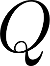 is the inverse of the CDF:

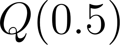 is the median, the value below which half the probability lies.
 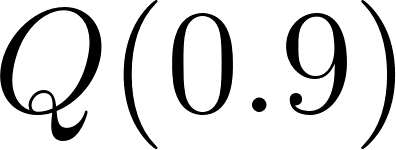 is the ninetieth percentile. Quantile functions are central to describing distributions in statistics; boxplots, confidence intervals, and value-at-risk calculations in finance all rely on quantiles. Note that the median and the mean are different in general. For symmetric distributions like the normal they coincide, but for skewed distributions like the exponential they can be very different.
Expectation and Variance for Continuous Variables
The definitions of expectation and variance carry over to the continuous case, with integrals replacing sums:
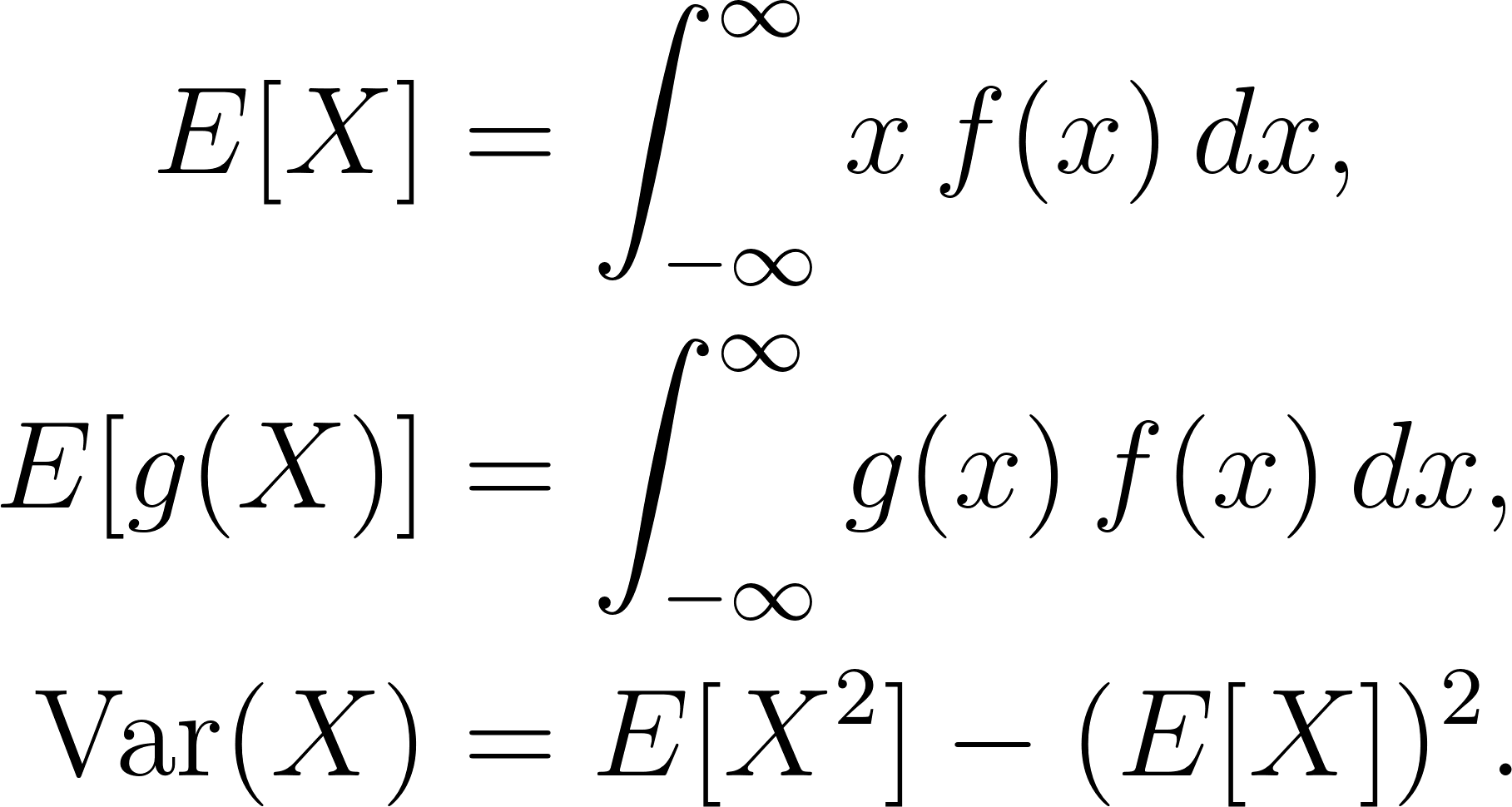
All the properties from the discrete case still hold: linearity of expectation, additivity of variance for independent variables, and the concentration inequalities of Markov and Chebyshev.
Numerical Integration
Since we cannot always compute integrals in closed form, the program uses numerical integration with the midpoint rule. The idea is to approximate the area under a curve by summing the areas of thin rectangles:
1 (defun integrate-rectangle (f a b &optional (n 100000))
2   "Approximate the integral of f from a to b via the midpoint rule
3    with N subintervals."
4   (let ((h (/ (- b a) n)))
5     (* h (loop for i from 0 below n
6                sum (funcall f (+ a (* h (+ i 1/2))))))))
With 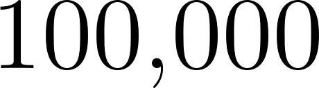 subintervals, this method is accurate enough for our purposes. The error of the midpoint rule decreases as
 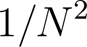 for smooth functions, so doubling the number of intervals reduces the error by a factor of
 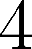 .
.
More sophisticated methods (Simpson’s rule, Gaussian quadrature, adaptive quadrature) achieve much higher accuracy for the same number of function evaluations, but the midpoint rule is easy to code, easy to reason about, and good enough for pedagogy. Numerical integration is the standard way to answer questions like “what is P(a <= X <= b)?” for any distribution whose CDF is not available in closed form.
To make the accuracy difference concrete, the program also includes Simpson’s rule, which fits a parabola to each pair of subintervals and has error 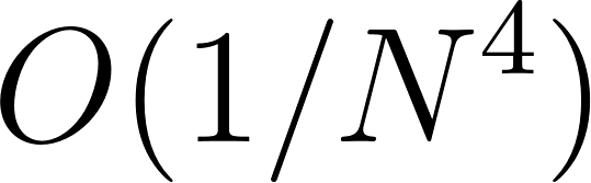 instead of
 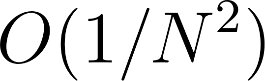 :
:
1 (defun integrate-simpson (f a b &optional (n 100000))
2   "Composite Simpson's rule: error O(1/N^4)."
3   (let* ((n (if (evenp n) n (1+ n)))
4          (h (/ (- b a) n))
5          (s (+ (funcall f a) (funcall f b))))
6     (loop for i from 1 below n
7           do (incf s (* (if (oddp i) 4.0d0 2.0d0) (funcall f (+ a (* i h))))))
8     (* (/ h 3.0d0) s)))
Integrating 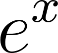 over
over 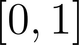 (exact value
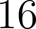
 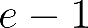 ) exposes the two convergence rates. Each time
 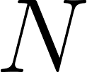 doubles, the midpoint error falls by about and the Simpson error by about
  :
:
1 === Numerical Integration: Midpoint vs Simpson ===
2   Integrating e^x over [0, 1] (exact = e - 1 = 1.718282):
3     n     midpoint error   Simpson error
4     4           4.467d-3        3.701d-5
5     8           1.118d-3        2.326d-6
6     16          2.796d-4        1.456d-7
7     32          6.992d-5        9.103d-9
8   Midpoint error falls ~4x per doubling (O(1/N^2)); Simpson ~16x (O(1/N^4)).
(The standard normal PDF is a poor test case for this comparison. Because that density and all its derivatives are essentially zero at the ends of a wide integration interval, the plain midpoint rule already converges extremely fast, and Simpson shows no clear advantage. The comparison needs an integrand with nonzero endpoint behaviour, such as .)
The Uniform Distribution
The uniform distribution on the interval 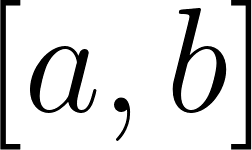 has a constant density:
 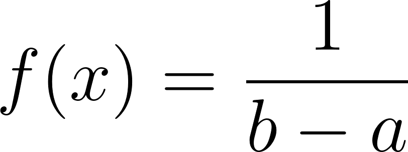 for
for 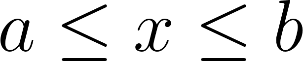 , and elsewhere. Every value in the interval is equally likely.

The mean is the midpoint of the interval, which makes sense by symmetry. The variance formula involves the factor 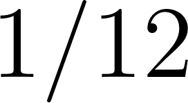 , which comes from integrating
 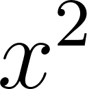 over against the flat density.
The uniform distribution plays a foundational role in probability:  random variables are the raw material from which nearly every random-number generator constructs other distributions. If
 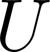 is uniform on and is the CDF of a distribution we want, then
 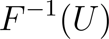 has that distribution. This is called the inverse-CDF method or inverse-transform sampling and it is behind much of the machinery of Monte Carlo simulation.
The program computes the mean both by formula and by numerical integration, and they match exactly:
1 === Uniform(0, 2) ===
2   E[X] (formula) =  1.0
3   E[X] (numeric) =  1.0
4   Var(X) (formula) = .333
5   P(0.5 <= X <= 1.5) =  0.5 (exact 0.5)
The Exponential Distribution
The exponential distribution with rate parameter 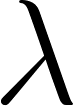 models waiting times in a Poisson process. Its PDF is:

The CDF has a simple closed form:  . The mean and variance are:

A higher rate means a shorter expected wait. If the rate is  , the expected wait is
 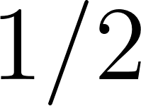 . The density decays exponentially, so most of the probability mass is concentrated near zero.
The exponential distribution shares the memoryless property with the geometric distribution. If you have been waiting for minutes, the distribution of the remaining wait time is still exponential with the same rate. The past does not affect the future.

The proof is a short computation. Since  ,
,

The exponential distribution is the only continuous distribution on 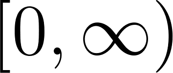 with this property, and its natural discrete counterpart is the geometric distribution. The link is exact in a limit: chop time into slices of width
 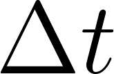 and let each slice be an independent Bernoulli trial with success probability
 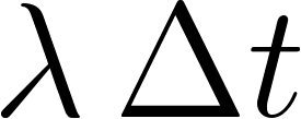 . The number of slices until the first success is geometric, and as
 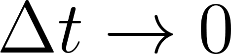 the waiting time converges in distribution to
  . The memorylessness of the geometric passes to the exponential in the limit.
The exponential distribution is closely related to the Poisson distribution we met briefly in the previous chapter. If events happen at random times such that the count of events in any interval of length  is Poisson with mean
 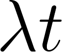 , and the counts in disjoint intervals are independent, then the time between successive events is exponential with rate . This unified picture is called the Poisson process and it describes radioactive decay, arrivals at a queue, and many other phenomena.
1 === Exponential(lambda=2) ===
2   E[X] (formula) =  0.5
3   E[X] (numeric) =  0.5
4   Var(X) (formula) = 0.25
5   P(X <= 1) = .865 (CDF) vs .865 (numeric)
6   Total probability (should be 1.0): .9999
The total probability comes out as 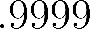 rather than a clean
 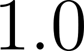 because we integrate only over
 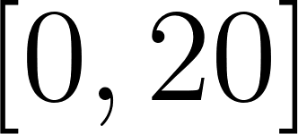 and the midpoint rule slightly underestimates the integral of a convex decreasing density. The missing mass is
  , so the shortfall we see is numerical, not a gap in the tail.
Sampling by Inverse Transform
The uniform distribution is also the raw material for generating samples from other distributions. The inverse-transform method takes a  draw and returns , which then has CDF . For the exponential, inverts to
  :
:
1 (defun sample-exponential (lambda-rate)
2   "Draw Exponential(lambda) by inverse transform: -ln(1-U)/lambda."
3   (/ (- (log (- 1.0d0 (random 1.0d0 *rng-state*)))) lambda-rate))
Drawing samples this way and computing their mean and variance recovers 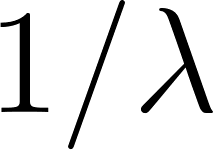 and
and 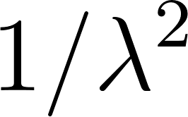 (Problem 5.8):
1 === Inverse-Transform Sampling: Exponential(lambda=2) ===
2   Drew 100000 samples via -ln(1-U)/lambda.
3   empirical mean = .50123  (1/lambda   =    0.5)
4   empirical var  = .25369  (1/lambda^2 =   0.25)
The exact figures shift from run to run because the samples are random, but they cluster around 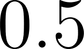 and
and 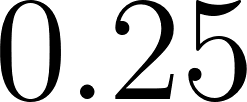 .
.
The Normal Distribution
The normal distribution (also called the Gaussian distribution) is the most important distribution in all of probability theory. Its PDF is the famous bell curve:

The parameter  is the mean (the center of the bell) and
 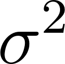 is the variance (how wide the bell is). The standard normal has
 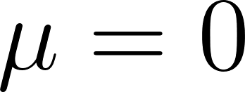 and
and 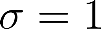 .
.
The normal distribution is universal: it appears as the limiting distribution of sums of independent random variables (the Central Limit Theorem in Chapter 7), as the maximum-entropy distribution given fixed mean and variance, and as the equilibrium distribution of many diffusive physical processes. Its density is smooth, symmetric, and unimodal, and it has the pleasant property that a sum of independent normals is again normal.
1 (defun normal-pdf (mu sigma x)
2   "PDF of Normal(mu, sigma^2): the bell curve."
3   (let ((z (/ (- x mu) sigma)))
4     (/ (exp (- (/ (* z z) 2.0)))
5        (* sigma (sqrt (* 2.0 pi))))))
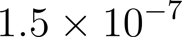
The normal CDF does not have a closed form in terms of elementary functions. It is written through the error function (erf) by the identity  . The program approximates erf with a rational-times-Gaussian formula from Abramowitz and Stegun (7.1.26), whose absolute error is below
  :
:
 1 (defun standard-normal-cdf (x)
 2   "CDF of the standard normal, Phi(x) = 0.5 (1 + erf(x / sqrt 2)), using the
 3    Abramowitz & Stegun 7.1.26 approximation to erf."
 4   (let* ((sign (if (>= x 0) 1 -1))
 5          (z (/ (abs x) (sqrt 2.0d0)))       ; erf argument: |x| / sqrt 2
 6          (t-val (/ 1.0 (+ 1.0 (* 0.3275911d0 z))))
 7          (y (* t-val (+ 0.254829592d0
 8                        (* t-val (+ -0.284496736d0
 9                                    (* t-val (+ 1.421413741d0 ...)))))))
10          (erf (- 1.0 (* y (exp (- (* z z)))))))
11     (* 0.5 (+ 1.0 (* sign erf)))))
The 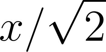 scaling is what turns the error function into the standard normal CDF; without it the code would return the CDF of a normal with variance . The modern successor to Abramowitz and Stegun is the NIST Digital Library of Mathematical Functions at dlmf.nist.gov.
The Moment Generating Function of the Normal
The normal distribution has moment generating function

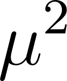
Differentiating at 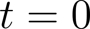 returns the mean , and the second derivative, after subtracting
  , returns the variance . The exponential-of-a-quadratic shape explains two facts stated above. First, if
  and
and  are independent, then multiplying their MGFs adds the exponents,

which is again a normal MGF, so  . The family is closed under adding independent members: means add and variances add. Second, an affine map
 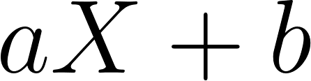 is normal with mean
 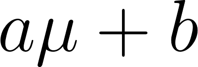 and variance
 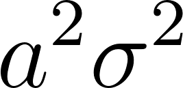 ; the special case
  is the standardization that turns any normal into the standard normal. This closure under sums and affine maps is exactly what makes the normal the natural limit in the Central Limit Theorem of the next chapter.
The 68-95-99.7 Rule
For any normal distribution, approximately:
- 68% of the probability mass lies within standard deviation of the mean
- 95% lies within standard deviations
- 99.7% lies within
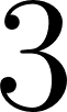 standard deviations
The program verifies this rule two independent ways: by integrating the PDF over each interval, and by differencing the standard-normal-cdf at the interval endpoints. The two columns agree:
1 === Standard Normal (mu=0, sigma=1) ===
2   E[X] (numeric) =    0.0 (should be 0)
3   E[X^2] (numeric) =    1.0 (should be 1 = Var)
4   Total probability (should be 1.0):  1.0
5   68% rule   P(-1<=Z<=1) = .683 (integ) .683 (CDF)  (~0.6827)
6   95% rule   P(-2<=Z<=2) = .954 (integ) .954 (CDF)  (~0.9545)
7   99.7% rule P(-3<=Z<=3) = .997 (integ) .997 (CDF)  (~0.9973)
8   CDF(0) =  0.5 (should be 0.5 by symmetry)
The two methods matching is a useful check on both: the integration and the closed-form CDF approximation are computed by completely different code, yet they land on the same 68-95-99.7 figures. The CDF at is exactly because the standard normal is symmetric about its mean of .
Other Named Continuous Distributions
Beyond the uniform, exponential, and normal, several other distributions appear frequently in probability and statistics. This list is not exhaustive but gives a sense of the broader landscape.
The Gamma distribution generalizes the exponential: it models the total waiting time until the 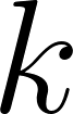 -th event in a Poisson process. When
 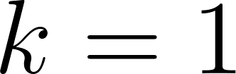 it is the exponential. When is a positive integer it is sometimes called the Erlang distribution.
The Beta distribution on the interval has two shape parameters  and
and 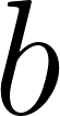 . It can be flat (
 , the uniform), symmetric (
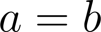 ), or heavily skewed (very different and ). The Beta is the conjugate prior for the Bernoulli likelihood in Bayesian inference, as we will see in Chapter 9.
The Chi-squared distribution with degrees of freedom is the distribution of a sum of squares of independent standard normals. It appears in hypothesis testing (chi-squared tests) and in confidence intervals for the variance of a normal.
The Student’s t distribution with degrees of freedom appears when estimating the mean of a normal population from a small sample. For large it is nearly the standard normal; for small it has heavier tails.
The log-normal distribution is the distribution of 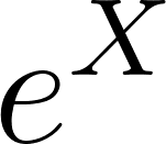 where is normal. It has a long right tail and is often used to model quantities that are positive and heavy-tailed, such as file sizes or income distributions.
These distributions form an interconnected web: many can be derived from one another by transformations, sums, or limits. Learning them one by one is less useful than understanding the general framework of PDFs, CDFs, expectations, and variance; the specific formulas become recognizable applications of a few underlying ideas.
The Maximum Entropy Viewpoint
A single principle picks out all three of our main distributions at once. The differential entropy of a continuous distribution with density 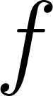 is
is

a measure of how spread out, or how uncommitted, the distribution is. Among all distributions consistent with a given set of constraints, the one that maximizes 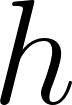 is the least presumptuous choice: it adds no structure beyond what the constraints force. The three workhorse distributions are exactly these maximum-entropy answers:
- Constrained only to live on a bounded interval, the maximum-entropy distribution is
 .
.
- Constrained to with a fixed mean, it is the
 distribution.
- Constrained to the whole real line with a fixed mean and variance, it is the
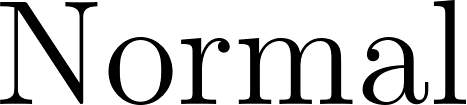 distribution.
This is why the three appear so often. Each is the most honest distribution to assume when all you know is a support, a mean, or a mean and a variance. The maximum-entropy principle recurs throughout statistical physics, information theory, and Bayesian modeling as a systematic way to turn partial knowledge into a full distribution.
Transformations of Random Variables
If is continuous with PDF 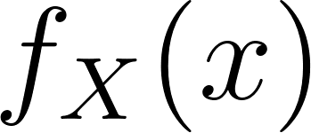 and
and 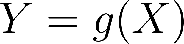 for a strictly increasing function
  , then the CDF of
 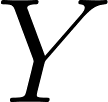 is
is  , and the PDF of is:

The absolute-value derivative is called the Jacobian of the transformation. This change-of-variables formula is essential for turning problems about one random variable into problems about another. For instance, the CDF of a squared standard normal can be derived from this formula, leading directly to the chi-squared distribution with degree of freedom.
Why This Matters
The uniform, exponential, and normal distributions are the three most commonly encountered continuous distributions. The uniform distribution is the simplest: flat and unconstrained. The exponential distribution models waiting times and decay processes. The normal distribution appears everywhere, thanks to the Central Limit Theorem that we will study in a later chapter. Understanding their PDFs, CDFs, means, and variances gives you the toolkit for working with continuous probability models.
Problem Set
Problem 5.1. Verify by numerical integration that the PDF of  integrates to over its support. Then compute
  both directly and using the uniform CDF, and confirm the two answers match.
Problem 5.2. For the exponential distribution with rate 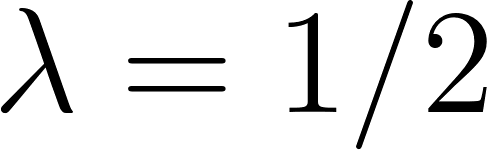 , use the CDF to compute
 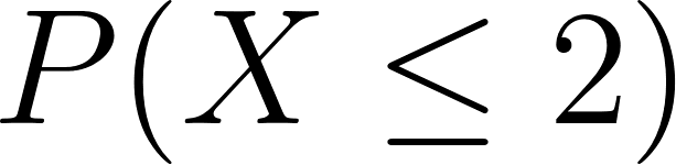 ,
, 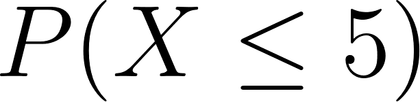 , and
, and  . Confirm your answers by numerical integration of the PDF.
Problem 5.3 (Memoryless property). For an exponential distribution with rate 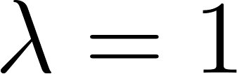 , verify by numerical calculation that
  equals
 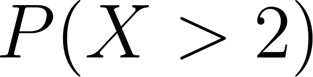 . Then prove the general identity
  using the CDF.
Problem 5.4 (Standard normal probabilities). Using the program’s standard normal CDF function, compute the following:
 (this is the critical value for a 95% two-sided confidence interval)
 (should be about
 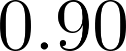 )
)
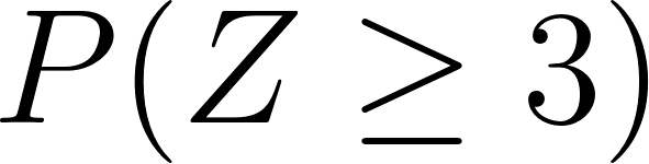 (a “three sigma” event)
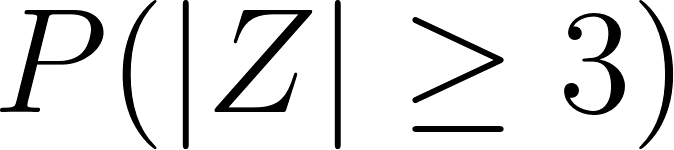 (the two-sided version)
Problem 5.5 (Converting normal to standard normal). Let be  (a common model for IQ scores). Using standardization , compute
  ,
,  , and the value such that
  .
.
Problem 5.6 (Median vs. mean). For the exponential distribution with rate , compute the median (the value 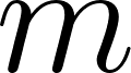 such that
  ). Compare it to the mean . Which is larger, and why does the exponential have this asymmetry?
Problem 5.7 (Numerical integration accuracy). Rerun the numerical integration of the standard normal PDF over 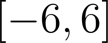 using
using  , and
, and 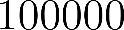 subintervals. Record the total integral in each case and note how quickly it converges to . Empirically, how does the error scale with the number of subintervals?
Problem 5.8 (Inverse-CDF sampling). Add a function sample-exponential to the example program that takes a rate and returns a sample from the exponential distribution using the inverse-CDF method: draw from and return  . Sample
 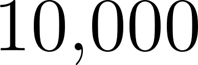 values, compute their empirical mean and variance, and compare against and .
Problem 5.9 (A transformation). Let 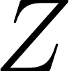 be a standard normal. Let
 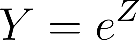 . What are the possible values of ? Using the change-of-variables formula, derive the PDF of . This is the standard log-normal distribution. Draw a rough sketch of its shape.