Monte Carlo Methods

Some quantities are easy to describe but hard to compute exactly. The Monte Carlo approach is to estimate them by repeated random sampling. The theoretical justification is the Law of Large Numbers: if we can express a quantity as an expectation, then the sample average of repeated random draws converges to that expectation.

The example program for this chapter is in the file 08_monte_carlo.lisp.

The idea of using random sampling to estimate mathematical quantities has surprisingly deep roots. In 1777, the French naturalist Georges-Louis Leclerc, Comte de Buffon, posed a problem about dropping a needle onto a floor of parallel lines and computed the probability that the needle crosses a line. His answer involved pi, giving an early example of a randomized geometric estimator for a mathematical constant.

The modern practice of Monte Carlo methods was developed in the 1940s at Los Alamos National Laboratory by Stanislaw Ulam, John von Neumann, and Nicholas Metropolis, in the context of the Manhattan Project. They needed to solve integrals arising in neutron transport that had no analytic solution, and Ulam suggested simulating the neutron trajectories randomly on the ENIAC computer. The name “Monte Carlo” was chosen by Metropolis as a nod to Ulam’s uncle, who often gambled at the Monte Carlo casino in Monaco.

Since then, Monte Carlo methods have become one of the most important computational techniques in all of science. They power simulations in physics, chemistry, biology, finance, engineering, and machine learning. The Markov chain Monte Carlo methods that underlie modern Bayesian statistics are direct descendants of the original Los Alamos work.

A Monte Carlo estimator works as follows. We want to estimate some quantity . We find a random variable whose expected value equals . Then we draw many independent samples of and average them:

By the Law of Large Numbers, converges to as grows. The variance of the estimator is , so the standard error decreases as 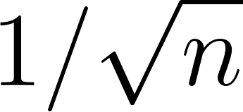. By the Central Limit Theorem, is approximately normal for large , so we can construct confidence intervals for using the normal-based methods from Chapter 7.

The design freedom in Monte Carlo lies in choosing the random variable . Any random variable whose expectation equals is a valid estimator, but different choices have different variances and therefore different accuracies for the same sample size. Much of the theory of Monte Carlo is really about finding good .

Two properties make this estimator trustworthy. It is unbiased: 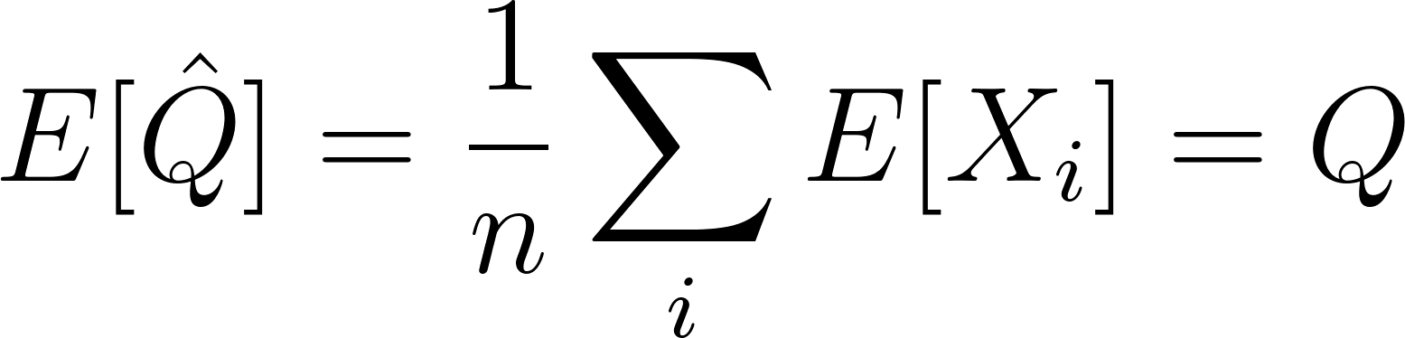for every , so it is centered on the right answer rather than merely approaching it. And because it is unbiased, its mean squared error equals its variance,

so the root-mean-square error is exactly the standard error 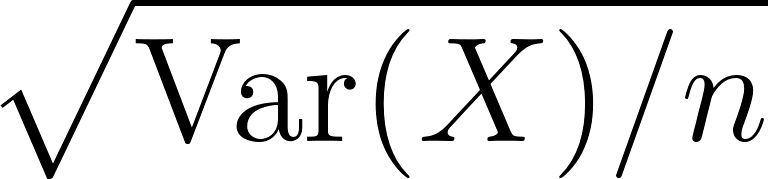that the program reports. Reducing error therefore means reducing , which is the whole point of the variance-reduction techniques below. Not every Monte Carlo estimator is unbiased, though: estimators built as ratios or other nonlinear functions of averages carry a bias of order 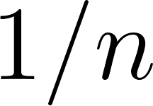, which the standard error dominates for large but which matters for small samples.

The most common use of the core idea is computing integrals, because any integral is an expectation in disguise. To evaluate

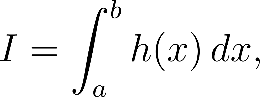
write it as with , since the uniform density on 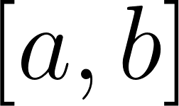is the constant 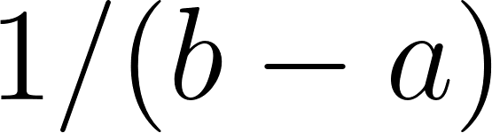. The estimator draws uniformly and averages:

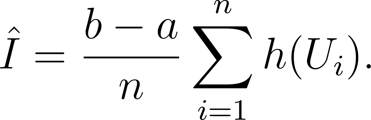
More generally, if 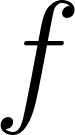is any density we can sample from, then , estimated by the plain average of 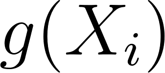over draws 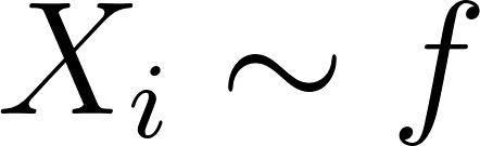. The choice of sampling density is where the design freedom lives, because the same integral can be rewritten against any density that is positive wherever the integrand is nonzero:

Sampling from an concentrated where is large is exactly the importance sampling we return to below; picking is the same as picking the estimator’s variance.

Our example estimates the value of . Consider a unit square (area ) and the quarter disk of radius centered at the origin (area 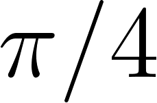). If we throw uniformly random points into the square, the probability that a point lands inside the quarter disk equals the ratio of the areas:

Let 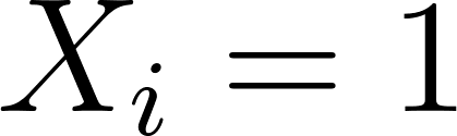if the 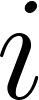-th point lands in the disk, otherwise. Then the 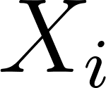are i.i.d. , and by the LLN:

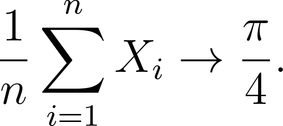
So our estimator is:

A point is inside the quarter disk if 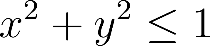, which is the Pythagorean distance from the origin. Uniform sampling over the square gives each region a probability equal to its area, which is the key property that makes the ratio of counts equal the ratio of areas.

How accurate is our estimate? For a variable, the standard error of the sample mean 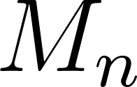is 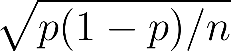. The estimator is 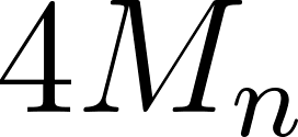, so its standard error is:

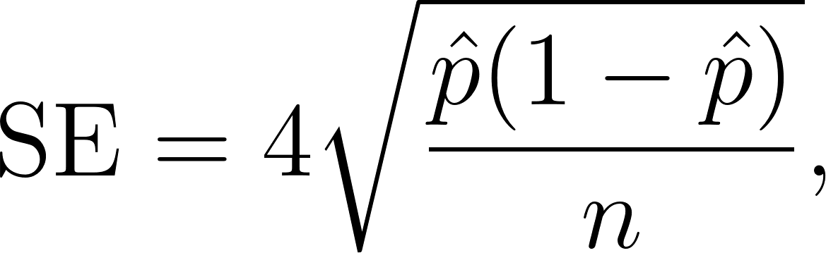
where 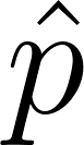is the sample proportion. The program reports both the estimate and the standard error:

By the Central Limit Theorem, an approximate 95% confidence interval for is . This lets us report the estimate along with a principled measure of its uncertainty.

With 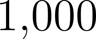points, the estimate is off by about . With 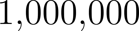points, the error drops to about . The standard error column tracks the actual error well: the error is typically within or standard errors of the true value. The random state is reseeded on each run, so your exact estimates will differ, while the shrinkage of the standard error stays the same.

The standard error decreases as . This is a slow convergence rate. To halve the error, you need times as many samples. To reduce the error by a factor of , you need times as many samples.

This is the fundamental tradeoff of Monte Carlo methods. They are incredibly general: you can estimate almost anything by random sampling. But they are slow to converge. For problems where exact computation is feasible, you should prefer exact methods. Monte Carlo shines when exact computation is intractable, such as high-dimensional integrals or complex probabilistic models.

An important observation: the rate does not depend on the dimension of the problem. Classical numerical integration (Simpson’s rule, Gaussian quadrature) has convergence rates that get worse in higher dimensions. In dimensions, deterministic quadrature typically has an error that scales like for some fixed depending on smoothness. When is large (say, ), this deterministic error decreases painfully slowly with the number of function evaluations. Monte Carlo, in contrast, still has the same rate regardless of dimension. This is why Monte Carlo dominates in high-dimensional problems like statistical physics, Bayesian inference in complex models, and reinforcement learning.

A large amount of Monte Carlo research is devoted to reducing variance without increasing the number of samples. Four common techniques:

Antithetic variates: pair each sample with its “opposite” so that variability partly cancels. For example, when sampling from , also use . If the estimator is monotonic in , the two are negatively correlated and their average has lower variance.

Control variates: subtract a related quantity whose expectation is known. If we want and know exactly, we can estimate for a well-chosen . If and are correlated, the modified estimator has lower variance.

Importance sampling: sample from a different distribution and reweight. Especially useful when the region of interest (say, a tail event) has low probability under the natural distribution.

Stratified sampling: partition the sample space into strata and sample proportionally from each.

These techniques can dramatically improve Monte Carlo performance in practice, often by a factor of or more. In our example, we could use antithetic variates by pairing 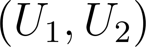with ; the correlation between the two indicator variables would reduce the variance of the estimator.

An alternative to true Monte Carlo is quasi-Monte Carlo, which uses low-discrepancy sequences like Sobol or Halton sequences instead of pseudo-random numbers. These sequences are more evenly spread than random points and can give convergence rates closer to rather than for smooth integrands. Quasi-Monte Carlo is widely used in high-dimensional finance and computer graphics, but its analysis is more delicate than classical Monte Carlo, and independence-based tools like the CLT do not apply directly.

Buffon’s original problem was to estimate the probability that a needle of length 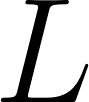dropped onto a floor with parallel lines spaced distance 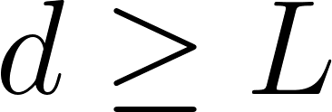apart will cross a line. Buffon showed that this probability is 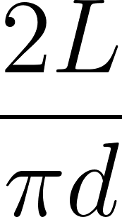. Rearranging, a Monte Carlo estimate of from dropped needles that produce 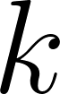crossings is:

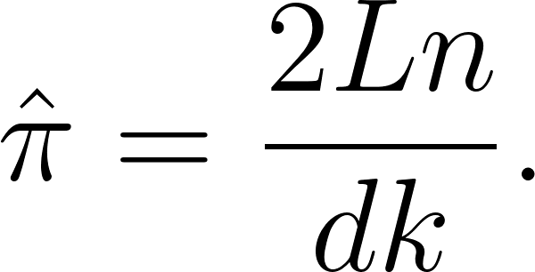
This is an even older and just as valid Monte Carlo estimator for as the disk method. It has different variance properties and is a nice teaching example.

The program implements both the antithetic-variates trick and Buffon’s needle, then compares three estimators by repeating each one times and reporting the empirical standard deviation of the estimates:

The antithetic estimator has a smaller standard deviation than the plain one at the same cost, so pairing each 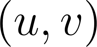with its reflection genuinely reduces variance (Problem 8.6). Buffon’s needle, using the same number of random draws, has the largest standard deviation of the three: a valid estimator but a less efficient one (Problem 8.4). The exact numbers vary from run to run.

Monte Carlo methods are used in physics (particle transport simulations), finance (option pricing), engineering (reliability analysis), and machine learning (Bayesian inference, reinforcement learning). The basic idea is always the same: express the quantity of interest as an expectation, then estimate it by averaging random samples.

Some concrete examples:

• Physics: simulate the trajectories of neutrons in a nuclear reactor to estimate the fraction that escape without absorption.
• Finance: simulate future price paths of an underlying asset to estimate the price of a complex option, especially path-dependent options.
• Machine learning: use Monte Carlo to approximate Bayesian posterior distributions in models where the posterior has no closed form (Markov chain Monte Carlo, particle filters).
• Statistics: bootstrap to estimate the variability of a sample statistic without needing a parametric model.
• Computer graphics: path tracing algorithms estimate the integral of light over all paths from a scene to the camera.

The estimation example is pedagogically simple, but the same principle scales to problems of enormous complexity. The only requirement is that you can simulate the random variable whose expectation you want. Once you can do that, the Law of Large Numbers does the rest, and the Central Limit Theorem tells you how uncertain your estimate is.

Problem 8.1. Run the example program with sample points. Record the standard error at each step and verify that it shrinks by roughly the factor of you would expect (since sample size quadruples each time and SE scales as ).

Problem 8.2 (Reproducibility). Modify the example to accept an optional seed for the random state and use it to reproduce the same estimate multiple times. Why is reproducibility particularly important in scientific Monte Carlo work?

Problem 8.3 (Estimating an integral). Use Monte Carlo to estimate 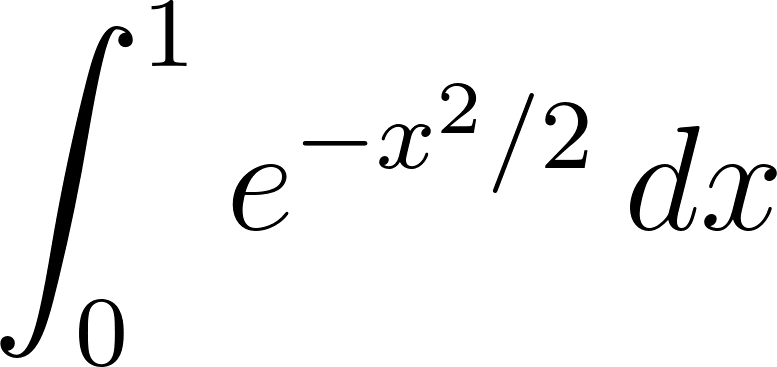. Compare against the exact value, which is where is the standard normal CDF. What sample size do you need to get within of the true answer with 95% confidence?

Problem 8.4 (Buffon’s needle). Implement Buffon’s needle in Common Lisp. Drop a needle of length onto a floor with lines spaced apart. Estimate from drops and report the standard error. Compare the accuracy to the disk method with the same .

Problem 8.5 (Volume of a d-dimensional ball). Use Monte Carlo to estimate the volume of the unit ball in 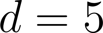dimensions. The exact answer is 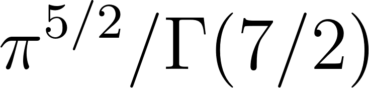, roughly . Now try and 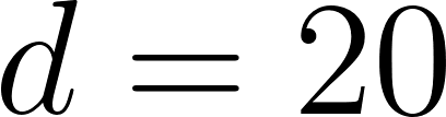. As grows, most of the volume of the enclosing hypercube lies outside the ball, so the naive Monte Carlo estimator becomes very inefficient. Comment on your observations.

Problem 8.6 (Antithetic variates). Modify the estimator to use antithetic variates: for each random , also use . Report the estimate and standard error. Compare against the plain estimator with the same total sample size.

Problem 8.7 (Confidence interval). For sample points in the estimation, report a 95% confidence interval for using the CLT-based formula . Does the true lie inside your interval?

Problem 8.8 (High-dimensional integration). Use Monte Carlo to estimate the average value of the function 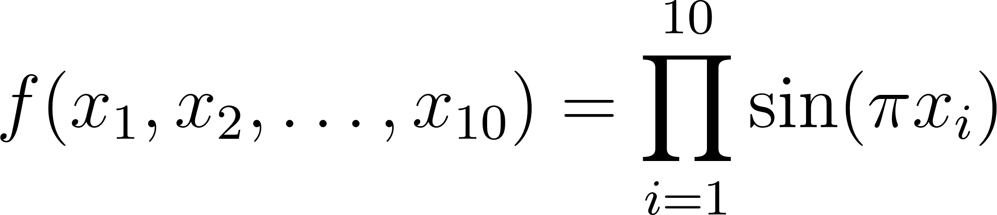over the unit hypercube . The exact answer is 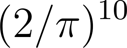. Compare the Monte Carlo estimate against a direct grid-based numerical integration attempt.

Problem 8.9 (Coding exercise). Add a general function monte-carlo-mean that takes a thunk (a function of zero arguments returning a sample) and a sample size , and returns the estimated mean along with a 95% confidence interval using the CLT. Test it on the disk indicator for and on the exponential from previous chapters.