Markov Chains
Many random processes unfold over time: the weather changes day by day, a stock price moves tick by tick, a customer navigates through a website page by page. A Markov chain is the simplest model for such sequential randomness. It captures the idea that the future depends on the present but not on the distant past.
The example program for this chapter is in the file 10_markov_chains.lisp.
Andrey Markov and the Origin of Markov Chains
The Russian mathematician Andrey Markov introduced these chains in 1906 as a way to study sequences of random variables that are not independent. Independence had been the dominant assumption in classical probability theory (as in Bernoulli’s theorem and the Central Limit Theorem), but many real phenomena are far from independent. Markov wanted to find the weakest form of dependence for which the great theorems of probability could still be proved.
His original motivating example was surprisingly literary: he analyzed the sequence of consonants and vowels in Pushkin’s novel-in-verse Eugene Onegin. He found that consonants and vowels are not independent: a vowel is more likely to be followed by a consonant than by another vowel. But he could still describe the sequence with a two-state Markov chain and could prove a version of the Law of Large Numbers for it. This was the birth of a new branch of probability theory.
Markov chains have since found applications in essentially every scientific field. Statistical mechanics, queueing theory, population genetics, computer science, natural language processing, and machine learning all use Markov chains as fundamental modeling tools.
The Markov Property
A Markov chain is a sequence of random variables  taking values in a state space. The defining property is the Markov property:

The next state depends only on the current state, not on the history of how we got there. This is sometimes called “memorylessness of the future given the present.”
The Markov property is a very strong assumption. It says that the current state contains all the information needed to predict the future. In a weather model, this would mean that today’s weather (Sunny or Rainy) tells us as much about tomorrow’s weather as any longer history. In reality, richer models could take into account humidity, pressure, season, and so on, but the Markov idealization is often a useful approximation.
When the Markov property does not hold in the raw data, a common trick is to expand the state space: define the state to include enough recent history that the resulting sequence is Markovian. For example, a language model that depends on the last two words can be seen as a Markov chain whose “state” is a pair of consecutive words.
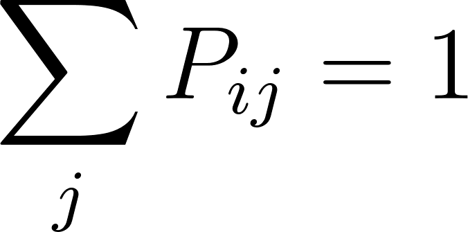
For a finite state space, the chain is described by a transition matrix 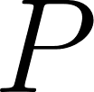 , where the entry
 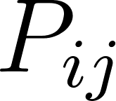 is the probability of moving from state
 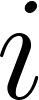 to state
 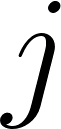 in one step. Each row of is a probability distribution: the entries are non-negative and
  .
.
A Weather Model
Our example uses a simple weather model with two states: Sunny and Rainy. The transition matrix is:
- From Sunny: 80% chance of staying Sunny, 20% chance of becoming Rainy
- From Rainy: 40% chance of becoming Sunny, 60% chance of staying Rainy
1 (let* ((P (make-transition-matrix
2             '((0.8 0.2)   ; from Sunny: 80% stay Sunny, 20% -> Rainy
3               (0.4 0.6)))) ; from Rainy: 40% -> Sunny, 60% stay Rainy
4        (start #(1.0d0 0.0d0)))  ; start certainly Sunny
5   ...)
If today is Sunny, there is an 80% chance tomorrow is Sunny too. But if today is Rainy, there is still a 40% chance of a Sunny tomorrow. The weather has persistence: Sunny days tend to follow Sunny days, and Rainy days tend to follow Rainy days.
Evolving the Distribution
If the state distribution at time  is a row vector
 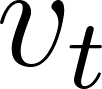 , then one step of the chain is a matrix multiplication:

After  steps, the distribution is
 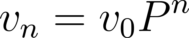 . The program computes this by repeated multiplication:
 1 (defun step-distribution (dist P)
 2   "Advance one step: v_{t+1} = v_t P. Returns a new distribution vector."
 3   (let* ((n (length dist))
 4          (result (make-array n :initial-element 0.0d0)))
 5     (dotimes (j n)
 6       (setf (aref result j)
 7             (reduce #'+ (loop for i below n
 8                               collect (* (aref dist i) (aref (aref P i) j))))))
 9     result))
10
11 (defun iterate-chain (dist P steps)
12   "Compute v_steps = v_0 P^steps by repeated multiplication."
13   (let ((d (copy-seq dist)))
14     (dotimes (s steps)
15       (setf d (step-distribution d P)))
16     d))
The -step transition matrix 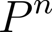 has a direct probabilistic meaning: the
 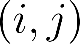 entry is
  , the probability of being in state after steps starting from state . Powers of the transition matrix are one of the primary computational objects when working with Markov chains.
These powers compose in the obvious way. The Chapman-Kolmogorov equations state that
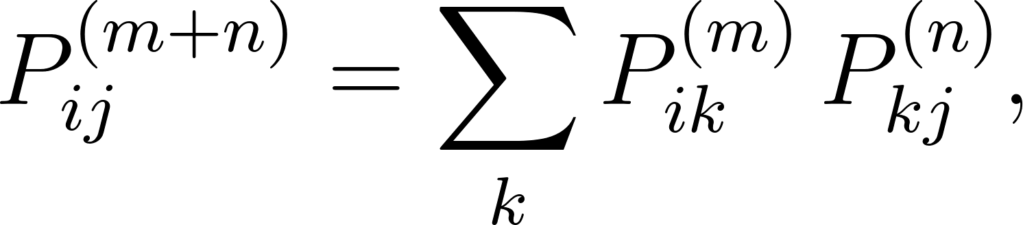
which is just  read entry by entry: to travel from to in
 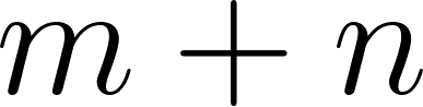 steps, pass through some intermediate state
 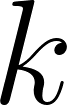 at time
 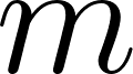 and sum over all the ways to do it. This identity is the Markov-chain backbone, and it is the discrete-state ancestor of the same-named equations that govern continuous-time and continuous-state Markov processes.
Classification of States
Not every state in a Markov chain behaves the same way. A rich vocabulary describes the possible behaviors.
A state communicates with state if there is a positive-probability path from to and from to . Communication is an equivalence relation; the state space partitions into communicating classes. A chain is irreducible if it has just one communicating class, meaning every state can eventually reach every other.
A state is recurrent if the chain returns to it with probability 1, and transient otherwise. In a finite Markov chain, recurrence is equivalent to the state being reachable from itself in the long run.
A state is absorbing if once the chain enters it, it never leaves. In matrix terms, an absorbing state has a  on the diagonal of . Absorbing chains have their own rich theory, useful for modeling processes that eventually terminate.
The period of a state is the greatest common divisor of the return times to that state. A state is aperiodic if its period is . Aperiodicity means the chain does not get locked into a deterministic cycle. A chain is ergodic if it is irreducible and aperiodic.
Our weather chain is both irreducible (Sunny and Rainy each reach the other) and aperiodic (the chain can stay in the same state, so no forced cycles). It is therefore ergodic, which as we will see next gives it a unique long-run behavior.
The Stationary Distribution
A stationary distribution  is a row vector that satisfies:
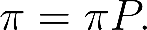
If the chain starts distributed as , it stays distributed as forever. The stationary distribution is a fixed point of the chain’s evolution.
For an irreducible chain (you can get from any state to any other state) that is aperiodic (not locked into a deterministic cycle), the stationary distribution exists, is unique, and the chain converges to it from any starting state:

This is the ergodic theorem for Markov chains. No matter where you start, the chain eventually settles into its equilibrium distribution. It generalizes the Law of Large Numbers: the long-run fraction of time the chain spends in state is 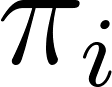 , regardless of the starting state.
Detailed Balance and Reversibility
A stronger condition than the stationarity equation 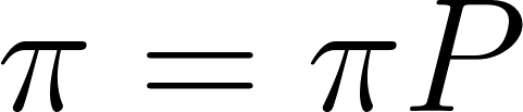 is detailed balance:

If and satisfy detailed balance, then is a stationary distribution (summing over gives the ordinary stationarity equation). A chain that satisfies detailed balance is called reversible: viewed in reverse time, it has the same statistical properties.
Detailed balance is a much easier condition to check than the full stationarity equation. Many designed Markov chains, especially those used in Markov chain Monte Carlo, are constructed to satisfy detailed balance for a target distribution .
Finding the Stationary Distribution
The program finds the stationary distribution two ways. The first is by long iteration: just run the chain for 10,000 steps and read off the distribution:
1 (defun stationary-by-iteration (dist P steps)
2   "Approximate the stationary distribution by long-run simulation of v_t P."
3   (iterate-chain dist P steps))
The second is by solving the linear system directly. For a two-state chain with transition matrix 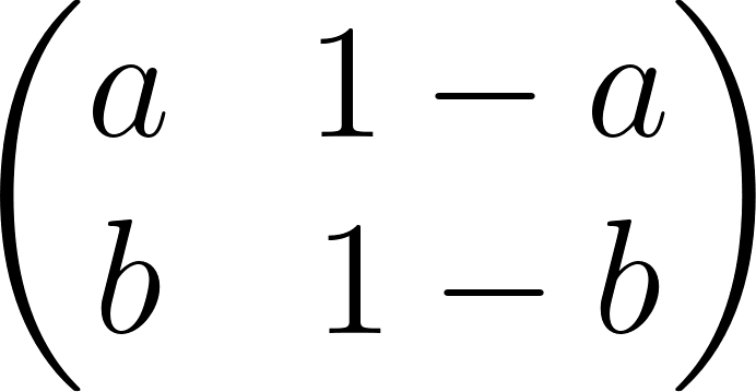 , the stationary distribution is:
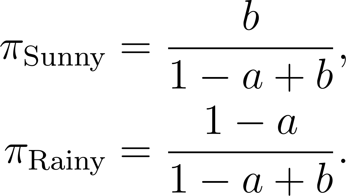
1 (defun stationary-by-linear-system (P)
2   "Solve pi = pi P exactly for a 2-state chain."
3   (let* ((a (aref (aref P 0) 0))   ; P[S->S]
4          (b (aref (aref P 1) 0))   ; P[R->S]
5          (denom (+ (- 1 a) b)))
6     (vector (/ b denom) (/ (- 1 a) denom))))
For larger chains, we solve the system  subject to the constraint
 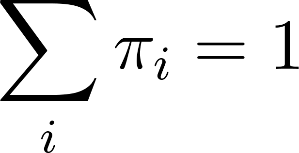 . This is a standard linear algebra problem and can also be posed as finding the left eigenvector of corresponding to eigenvalue .
Why the Chain Converges: The Spectral View
Why should 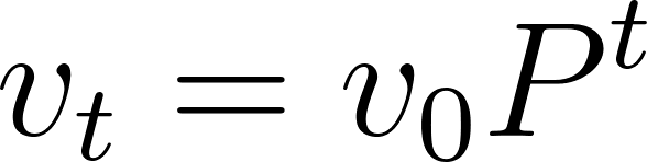 settle down at all, and how fast? The answer lives in the eigenvalues of . Because every row of sums to , the all-ones column vector is a right eigenvector with eigenvalue , so is always an eigenvalue of a stochastic matrix. The Perron-Frobenius theorem supplies the rest: for an irreducible, aperiodic stochastic matrix the eigenvalue is simple, with no repeats, and every other eigenvalue satisfies
 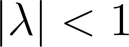 . The left eigenvector for eigenvalue , normalized to sum to , is the stationary distribution , and its uniqueness is exactly the simplicity of that eigenvalue.
Convergence then follows by expanding the starting distribution along the eigenvectors of . Writing the eigenvalues as  , the component along stays fixed while every other component is multiplied by its eigenvalue at each step:

since 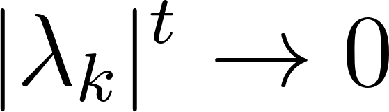 for
for 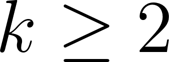 . The slowest-decaying term is governed by the second-largest eigenvalue modulus
 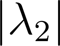 , often called the SLEM. The distance to stationarity shrinks geometrically at rate : a value near
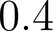
  means the chain forgets its start almost at once, a value near means slow mixing. For the weather chain the eigenvalues are and
  , so the deviation from
 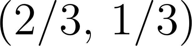 falls by a factor of each step, which is why the printed distribution has already reached equilibrium by step
 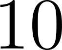 .
.
The natural way to measure the remaining gap is the total variation distance

the largest difference in probability the two distributions assign to any event. The mixing time is the number of steps needed to push this distance below a small  . Because the total variation distance decays like
 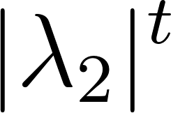 , the mixing time scales as
  up to constants. Controlling is the central problem in the design of Markov chain Monte Carlo samplers, where a chain that mixes slowly can make an otherwise correct algorithm useless in practice. Problems 10.9 and 10.10 measure this decay directly.
Running the Example
 1 === Markov Chain: Weather Model ===
 2 States: (Sunny Rainy)
 3 Transition matrix P (rows = from-state):
 4   Sunny -> [ 0.8,  0.2]
 5   Rainy -> [ 0.4,  0.6]
 6
 7 Start distribution: [1, 0] (certainly Sunny).
 8 Iterating v_{t+1} = v_t P:
 9   steps=0   : [1.0000, 0.0000]
10   steps=1   : [0.8000, 0.2000]
11   steps=2   : [0.7200, 0.2800]
12   steps=5   : [0.6701, 0.3299]
13   steps=10  : [0.6667, 0.3333]
14   steps=50  : [0.6667, 0.3333]
15   steps=100 : [0.6667, 0.3333]
16
17 Stationary distribution (by long iteration, t=10000):
18   [0.6667, 0.3333]
19 Stationary distribution (exact, 2-state closed form):
20   [0.6667, 0.3333]
21 Stationary distribution (general linear solve, any size):
22   [0.6667, 0.3333]
23
24 Convergence to stationarity (total variation distance to pi):
25   t=0    TV=0.3333
26   t=1    TV=0.1333
27   t=2    TV=0.0533
28   t=3    TV=0.0213
29   t=4    TV=0.0085
30   t=5    TV=0.0034
31   t=10   TV=0.0000
32 Mixing time (TV <= 0.01) starting from [1,0]: 4 steps
33
34 Simulating one 100000-step trajectory (start Sunny):
35   empirical P(Sunny) = 0.6627 (stationary 0.6667)
36
37 The chain forgets its initial state and converges to the
38 unique stationary distribution (ergodic theorem for Markov chains).
Watch the distribution evolve. We start certainly Sunny: [1, 0]. After one step, there is an 80% chance of Sunny and 20% of Rainy. After two steps, the distribution has shifted further: [0.72, 0.28]. By step 10, the distribution has settled at approximately [2/3, 1/3], and it stays there forever.
The stationary distribution is [2/3, 1/3]: in the long run, about 67% of days are Sunny and 33% are Rainy. All three methods of finding it agree: long iteration, the two-state closed form, and a general linear solve that works for any number of states (it sets up  with the last row replaced by the normalization and solves by Gaussian elimination).
The program also measures how fast the chain reaches equilibrium. The total variation distance to falls by a factor of at every step, which is exactly the second eigenvalue of predicted by the spectral view above, and the mixing time to get within 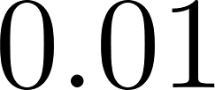 is
is 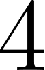 steps. A separate
 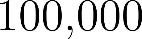 -step simulation of a single trajectory spends about
 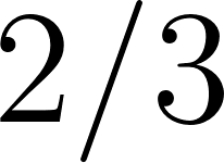 of its time in the Sunny state, the same
 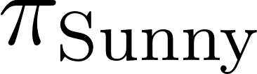 from a completely different computation (the exact fraction varies from run to run).
Hitting Times and First-Step Analysis
The stationary distribution answers questions about the long run. A different and equally practical question asks when something first happens: how many steps until the chain first reaches a state, or which of several absorbing states it ends up in. The standard tool is first-step analysis, which sets up equations by conditioning on the first transition, exactly the self-consistency trick we used for the geometric mean in Chapter 4.
Let 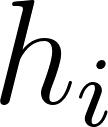 be the expected number of steps to reach a target set
 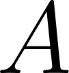 starting from state . If
 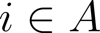 then
then 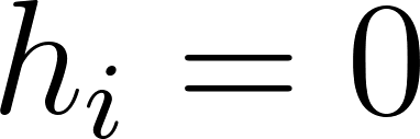 . Otherwise, conditioning on the first move,
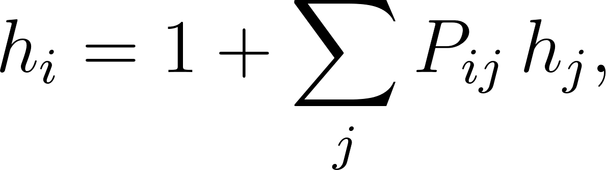
where the counts the step just taken and the sum averages the remaining time over where that step lands. This is one linear equation per state, and solving the system gives every expected hitting time at once. Absorption probabilities obey the same kind of system with the removed: if 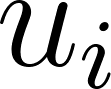 is the probability of ending at a chosen absorbing state starting from , then
 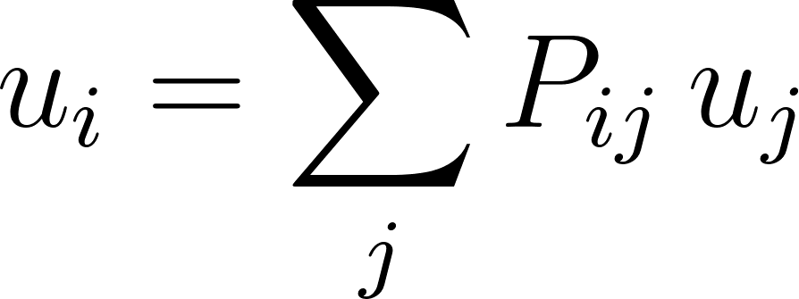 , with boundary values
 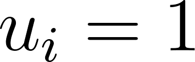 at that target and
 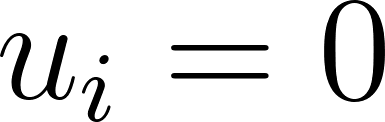 at the other absorbing states. First-step analysis is the workhorse behind Problems 10.5 and 10.7, and it is how one computes expected waiting times, gambler’s-ruin probabilities, and the expected running time of randomized algorithms.
Applications of Markov Chains
Markov chains model a vast range of real-world processes. A partial list:
PageRank. Google’s original algorithm for ranking web pages models the web as a huge Markov chain: at each step, a “random surfer” clicks a link on the current page, with occasional teleportation to a random page to guarantee irreducibility. The stationary distribution assigns high weight to pages that many random surfers spend time on. PageRank is a computation of this stationary distribution.
Queueing systems. In operations research, the number of customers in a queue often forms a Markov chain. Its stationary distribution tells us the long-run behavior of the queue: average wait times, server utilization, and so on.
Hidden Markov models. In speech recognition, bioinformatics, and finance, we often observe some quantity that depends on an underlying Markov chain we cannot directly see. Hidden Markov models let us infer the underlying states from the observations.
Reinforcement learning. Modern reinforcement learning is built on Markov decision processes, which extend Markov chains with actions and rewards. An agent chooses actions to maximize expected cumulative reward in an environment whose state evolves as a Markov chain conditional on the agent’s actions.
Markov chain Monte Carlo (MCMC). To sample from a complicated target distribution , we can construct a Markov chain whose stationary distribution is exactly and run it for a long time. The Metropolis-Hastings algorithm and Gibbs sampling are the two workhorses of MCMC. This has become the dominant computational tool of Bayesian statistics.
Statistical mechanics. The state of a physical system at thermal equilibrium is distributed according to the Boltzmann distribution, which is the stationary distribution of many physical Markov chains. MCMC and physics share deep intellectual roots.
Beyond Discrete Time
The Markov chains we have discussed evolve at discrete time steps. There is a parallel theory of continuous-time Markov chains, in which transitions happen at random times drawn from exponential distributions. Continuous-time Markov chains describe systems like radioactive decay, chemical reactions, and queueing systems.
There is also a theory of general Markov processes with continuous state spaces, culminating in stochastic differential equations and Brownian motion. These lie beyond the scope of this book, but they build on the same central intuition: the future depends on the present, not on the past.
Why This Matters
The stationary distribution is particularly important. It tells you the long-run behavior of the system: what fraction of time the chain spends in each state, regardless of where it started. This makes Markov chains a powerful tool for analyzing systems that reach equilibrium, from physical systems to computer networks to economic models.
The convergence to stationarity is also the foundation of Markov chain Monte Carlo, which has become the computational engine of modern Bayesian statistics and countless applications in machine learning. Understanding Markov chains is the entry point to a huge portion of modern probabilistic modeling.
Problem Set
Problem 10.1. For the weather chain with transition matrix 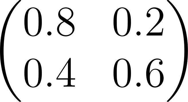 , verify by direct substitution that
  satisfies .
Problem 10.2 (Different starting state). Rerun the example program starting from 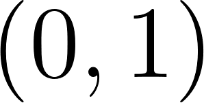 (certainly Rainy). Does the chain still converge to the same stationary distribution? By what step is the distribution effectively at equilibrium? Explain in words why the answer does not depend on the starting state.
Problem 10.3 (A three-state chain). Consider a chain over states A, B, C with transition matrix
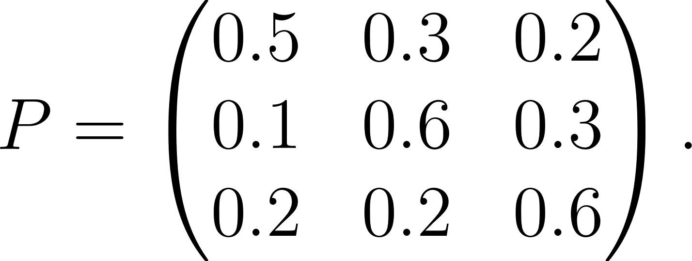
Extend the example program to handle three states and compute the stationary distribution by long iteration. Confirm your answer by verifying .
Problem 10.4 (Detailed balance). Does the two-state weather chain satisfy detailed balance for ? Check the condition  with numerical values. Every two-state chain with a stationary distribution satisfies detailed balance, so this should hold.
Problem 10.5 (An absorbing chain). Consider a chain over states 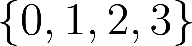 where state and state
 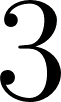 are absorbing (all transitions from them stay in place) and states and
  each transition to either neighbor with probability
 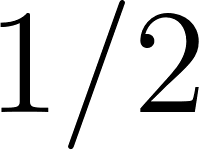 . Starting in state , compute the probability of eventually being absorbed at state versus state .
Problem 10.6 (Periodic chain). Consider a chain over states 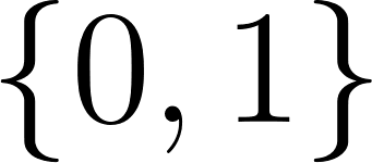 where state always transitions to state and state always transitions to state . Starting from
 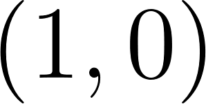 , iterate the chain. What do you observe? Explain why this chain does not converge to a stationary distribution, despite the fact that
 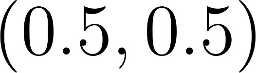 satisfies the stationarity equation.
Problem 10.7 (Expected hitting time). For the weather chain, starting Sunny, what is the expected number of days until the first Rainy day? Hint: the number of days is a geometric random variable with success probability 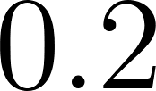 (from the Sunny to Rainy transition). Confirm this both by formula and by simulation.
Problem 10.8 (Simulating the chain). Modify the program to simulate one long trajectory of the weather chain: at each step, draw a uniform random number and use it to determine the next state given the current state. Run for 100,000 steps and compute the empirical fraction of Sunny days. Compare against the stationary probability .
Problem 10.9 (Convergence rate). For the weather chain, plot the total variation distance 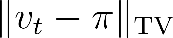 between the distribution at step and the stationary distribution, as grows from to
 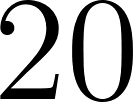 . How quickly does the distance shrink? The rate is controlled by the second eigenvalue of .
Problem 10.10 (Coding exercise). Add a function mixing-time that takes a Markov chain , a starting distribution, and a tolerance , and returns the smallest such that the total variation distance from stationarity is at most . Test it on the weather chain with 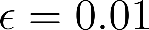 .
.