Conditional Probability

In the previous chapter we learned to compute probabilities by counting outcomes. But what happens when we gain partial information about an experiment? If we know that one event has occurred, does that change the probability of another event? The answer is yes, and the tool for reasoning about this is conditional probability.

The example program for this chapter is in the file 02_conditional_probability.lisp.

Almost every real-world probability question is really a conditional question. A doctor does not ask “what is the probability this patient has diabetes?” in the abstract. She asks “what is the probability this patient has diabetes given the observed symptoms and lab results?” A jury does not evaluate whether a defendant is guilty in a vacuum. It evaluates guilt given the evidence presented at trial. A weather forecaster does not report the marginal probability of rain averaged over all possible tomorrows; she reports the probability of rain given the current radar image and pressure readings.

Unconditional (or marginal) probabilities are useful as inputs, but almost all interesting reasoning is conditional. Learning to work fluently with conditional probability is the single most important skill in this book.

The conditional probability of event 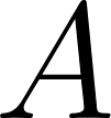given event 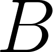, written 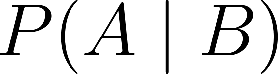, measures how likely is once we know that has occurred. The formula is:

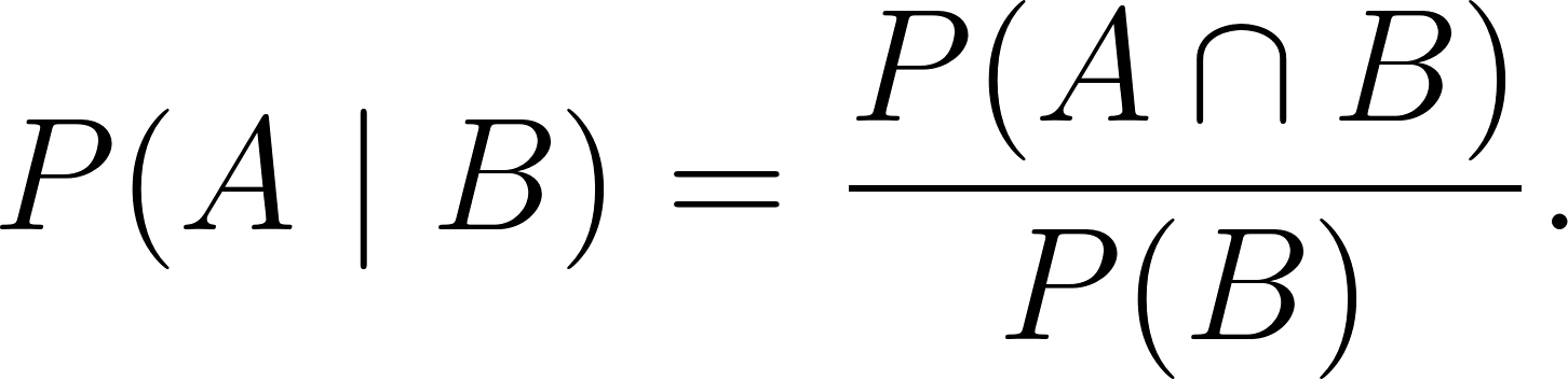
The intuition is that once we know happened, becomes our new sample space. We ask: what fraction of also contains ? The numerator is the probability that both and occur, and the denominator is the probability that occurs at all.

Note that is defined only when 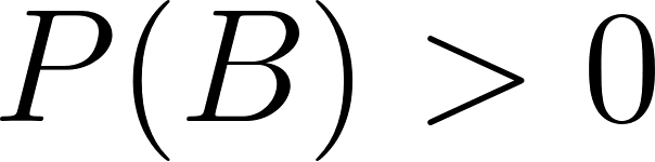. Conditioning on an event of probability zero is not meaningful in the discrete setting. There is a more elaborate theory of conditional expectation that handles the continuous case, but we will not need it.

In the example program, we compute conditional probability by taking the intersection of the two events and dividing by the size of the conditioning event:

1 (defun conditional-probability (a b omega)
2   "P(A | B) = P(A intersection B) / P(B).
3    The intersection A intersection B is the set of outcomes in BOTH events."
4   (let ((intersection (intersection a b :test #'equal)))
5     (/ (length intersection) (length b))))

An important sanity check: 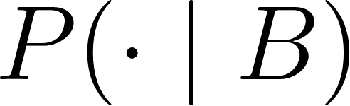is itself a bona-fide probability measure. Fixing and letting vary, the function satisfies all three Kolmogorov axioms on the sample space . Non-negativity is immediate; normalization holds because ; and additivity carries over from the additivity of 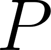. This means every theorem we know about probability measures applies equally well to conditional probabilities. In particular, the complement rule still holds.

Rearranging the definition of conditional probability gives the multiplication rule:

This is often the easiest way to compute the joint probability of two events. Rather than dealing with the intersection directly, you compute one probability and then a conditional probability.

Extending this to more events gives the chain rule of probability:

The chain rule is the backbone of most probabilistic model-building. Any complicated joint distribution can be factored into a product of simpler conditional distributions. Bayesian networks and hidden Markov models rely on this idea directly.

Two events and are independent if knowing one tells you nothing about the other. Formally, and are independent if and only if:

Equivalently, when and are independent. The condition does not change the probability.

Independence is one of the most important concepts in probability. Many powerful results, such as the Law of Large Numbers and the Central Limit Theorem, require independence as a hypothesis. Whenever you assume events are independent, you are making a real assumption about the world; whenever a proof assumes independence, that assumption is doing real work.

A common source of confusion is the difference between independent events and disjoint (mutually exclusive) events. These concepts are almost opposites.

Disjoint events cannot happen together: . If occurs, then cannot occur. So if we learn that occurred, we can be certain that did not, meaning that , not 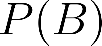. Disjoint events are highly dependent.

Independent events can happen together, and their joint probability is exactly the product 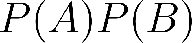. Learning that occurred does not change our estimate of .

Disjoint events with positive probability are never independent, and independent events with positive probability are never disjoint. This is worth pausing to internalize; many mistakes in probability come from confusing these two concepts.

In our two-dice example, the event “first die is 1” and the event “second die is 1” are independent because the two dice do not affect each other. But the event “first die is 1” and the event “sum is 7” are also independent, which is less obvious. Let us see why: if the first die is , the second die must be 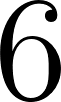for the sum to be 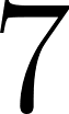, and that happens with probability 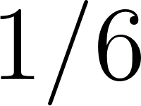, which is the same as the unconditional probability .

The program checks independence by comparing P(A and B) with P(A) times P(B):

1 (defun independent-p (a b omega)
2   "Are A and B independent?  Check whether P(A intersection B) = P(A) * P(B)."
3   (let ((intersection (intersection a b :test #'equal)))
4     (= (probability-classical intersection omega)
5        (* (probability-classical a omega)
6           (probability-classical b omega)))))

For three or more events the definition of independence becomes more subtle. Events , , and are mutually independent if the joint probability factors for every subset:

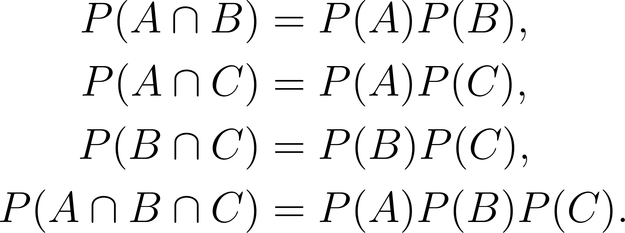
Pairwise independence (the first three conditions) does not imply mutual independence. There are classical examples of three events that are pairwise independent but for which the joint probability is not equal to the product . Whenever a theorem or model calls for “independent” events, it almost always means mutually independent.

Independence can hold or fail within a sub-population. Events and are conditionally independent given C$ if

Equivalently, : once we know , learning adds nothing further about . This is a different statement from ordinary (marginal) independence, and neither one implies the other. Two events can be dependent overall yet independent inside every stratum of , and two events independent overall can become dependent once we condition on .

Here is the intuition. Let and be the events that two different residents of a town test positive for the same infection. Marginally, and are dependent: a positive result for the first person raises our estimate that an outbreak is under way, which raises the chance the second tests positive too. But given the true prevalence in the town, the two results are independent, because fixing the common cause that linked them removes the link.

Conditional independence is the structural assumption behind the graphical models mentioned above. A naive Bayes classifier assumes the observed features are conditionally independent given the class label. A hidden Markov model assumes each observation is conditionally independent of the rest of the chain given its own hidden state. A Bayesian network is a compact encoding of a long list of such statements. Each assumption replaces one intractable joint distribution with a product of small factors, and the practical value of these models rests on it.

The law of total probability is a tool for decomposing a hard probability into simpler pieces. If partition the sample space (they are disjoint and cover everything), then for any event :

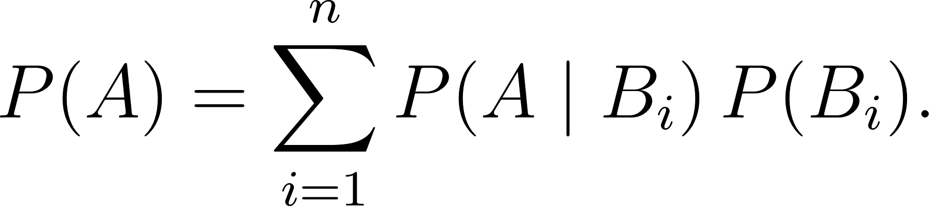
Each term answers the question: what is the probability of and 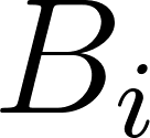happening together? Summing over all the accounts for all the ways can happen.

The law of total probability is often applied when you know the conditional probabilities 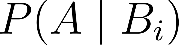and the probabilities 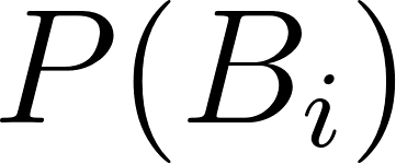of the pieces of the partition, but you do not directly know 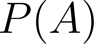. The formula stitches these together into a single number.

We will use this law in the next section to compute the denominator in Bayes’ theorem.

Bayes’ theorem is one of the most important results in probability theory. It tells us how to reverse the direction of conditioning. If we know , we can compute :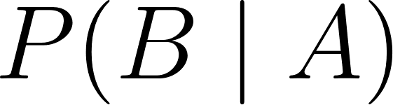

Here is called the prior: what we believed about before seeing evidence. is the likelihood: how likely the evidence is if is true. is the posterior: what we believe about after seeing the evidence. The denominator is computed using the law of total probability.

A more general form of Bayes’ theorem partitions the space with several hypotheses :

This is the form used in classification problems, where each represents a possible class label and represents the observed features.

There is an alternative and often more convenient form of Bayes’ theorem that works with odds instead of probabilities. The odds in favor of an event are defined as . In this form Bayes’ theorem becomes:

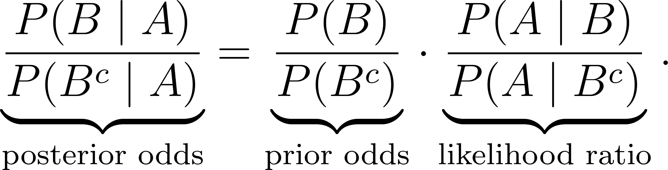
The likelihood ratio is . This form is elegant because the normalizing constant drops out. Doctors, forensic scientists, and information retrieval systems often work directly in log-odds; each new piece of evidence adds a constant amount to a running log-odds score.

The classic application of Bayes’ theorem is medical testing. Suppose we have a disease that affects 1% of the population. We have a test with 99% sensitivity (it correctly identifies 99% of sick people) and 95% specificity (it correctly identifies 95% of healthy people). If a person tests positive, what is the probability they actually have the disease?

Most people intuitively guess around 99%, but the answer is dramatically lower. Let us work through it:

 1 (defun bayes-medical-test ()
 2   (let* ((p-disease 1/100)            ; prior P(D)
 3          (p-healthy 99/100)           ; P(no D) = 1 - P(D)
 4          (p-pos-given-disease 99/100) ; likelihood P(+ | D)
 5          (p-pos-given-healthy 5/100)) ; likelihood P(+ | no D)
 6     ;; Total probability of a positive test:
 7     ;;   P(+) = P(+ | D) P(D) + P(+ | no D) P(no D)
 8     (let ((p-positive (+ (* p-pos-given-disease p-disease)
 9                          (* p-pos-given-healthy p-healthy))))
10       ;; Bayes: P(D | +) = P(+ | D) P(D) / P(+)
11       (let ((posterior (/ (* p-pos-given-disease p-disease) p-positive)))
12         ...))))

The prior probability of having the disease is only 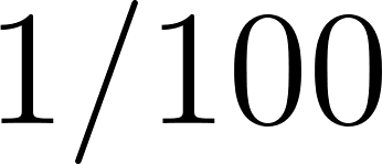. The test has a 5% false-positive rate, and since 99% of the population is healthy, those false positives add up. The total probability of a positive test is:

The posterior probability is:

So a positive test means only about a 16.7% chance of actually having the disease. This counterintuitive result arises because the disease is rare and false positives from the large healthy population dominate the true positives.

The medical-testing surprise illustrates the base rate fallacy, a widespread cognitive bias. When people evaluate evidence, they tend to focus on the likelihood and neglect the prior . The base rate (the prior) is easy to overlook, yet it dominates the calculation when the hypothesis is rare.

The same fallacy appears in criminal trials (the prosecutor’s fallacy, in which the probability of the DNA match given innocence is confused with the probability of innocence given the DNA match), in security screening (a very accurate test can still generate mostly false alarms when hunting for extremely rare threats), and in many other high-stakes settings. Understanding Bayes’ theorem is not just mathematically satisfying; it is a defense against widely-made real-world reasoning errors.

Conditioning can reverse the direction of an association. A treatment can raise the recovery rate in every subgroup of patients and still lower the recovery rate in the pooled data. This reversal is Simpson’s paradox, and it follows directly from the algebra of conditional probability.

Write 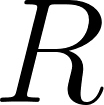for recovery, 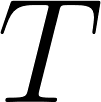for receiving the treatment, and for a covariate, say a severe case versus a mild one. It is possible to have the treatment win in both strata,

and yet lose overall,

Nothing is wrong with the arithmetic. By the law of total probability the pooled rate is a weighted average of the two subgroup rates,

and the treated and untreated groups can carry very different weights 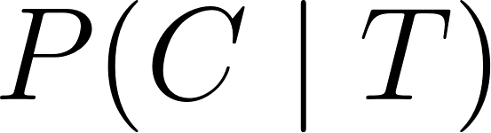and 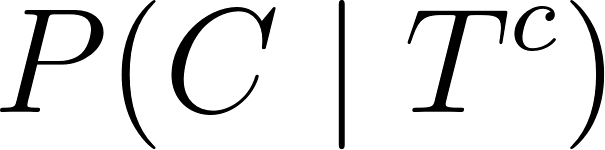. If the treatment went mostly to the severe cases, its overall rate is dragged down by that harder mix of patients even while it helps within each severity level.

The lesson is that 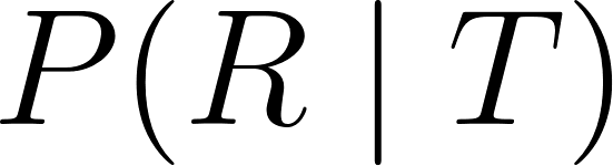and answer different questions, and only the second holds the confounder fixed. Deciding which one should guide a decision is the province of causal inference, a subject that begins exactly where this paradox does.

When you load the program, you see:

 1 === Conditional Probability with Two Dice ===
 2 
 3 B = 'first die is 1',  |B| = 6
 4 A = 'sum is 7',        |A| = 6
 5 P(A)         = 1/6 = .167
 6 P(A | B)     = 1/6 = .167
 7 Independent? yes
 8 
 9 e1 = 'first die is 1', e2 = 'second die is 1'
10 P(e1) = 1/6, P(e2) = 1/6, P(e1 ∩ e2) = 1/36
11 Independent? yes (rolling separate dice never affects each other)
12 
13 === Bayes' Theorem ===
14 
15 Medical screening example (Bayes' theorem):
16   Prior P(D)           = 1/100 = 0.01
17   Sensitivity P(+|D)   = 99/100 = 0.99
18   False-positive P(+|no D) = 1/20 = 0.05
19   Total P(+)           = 297/5000 = .059
20   Posterior P(D | +)   = 1/6 = .167
21   => A positive test means only 16.7% chance of disease!

The first part shows that equals when and are independent, confirming the theory. The second part demonstrates the surprising power of Bayes’ theorem to correct our intuitions about evidence and prior beliefs.

Conditional probability and Bayes’ theorem are the engines that power statistical inference, machine learning classification, spam filtering, medical diagnosis, and many other applications. Whenever you need to update your beliefs in light of new evidence, you are applying Bayes’ theorem, whether you realize it or not. In a later chapter we will see how Bayesian inference extends this idea to continuous updating of beliefs as data streams in.

Problem 2.1. For the two-dice sample space, let be the event “sum is 8” and be the event “first die is 4.” Compute , and . Are and independent? Give an intuitive explanation for your answer.

Problem 2.2. Two cards are drawn from a standard deck without replacement. Compute the probability that both are aces. Solve the problem two ways: (a) by counting the number of favorable ordered pairs and dividing by the total number of ordered pairs, and (b) by using the multiplication rule .

Problem 2.3 (Independence vs. disjointness). Give an example of two events on the two-dice sample space that are disjoint but not independent. Then give an example of two events that are independent but not disjoint. Explain why disjoint events with positive probability can never be independent.

Problem 2.4 (The Monty Hall problem). You are on a game show. There are three doors. Behind one door is a car; behind the other two are goats. You pick door 1. The host, who knows what is behind each door, opens door 3 to reveal a goat. He then offers you the chance to switch to door 2. Should you switch? Use Bayes’ theorem to compute the probability of winning if you switch and the probability of winning if you stay. Then modify the example program to simulate the game 100,000 times and empirically confirm your answer.

Problem 2.5 (The two-child problem). A family has two children. You are told that at least one of them is a boy. What is the probability that both are boys? (Assume boys and girls are equally likely and the sexes of the two children are independent.) Now suppose instead you are told that the older child is a boy. What is the probability that both are boys? Compare the two answers and explain why they differ.

Problem 2.6 (A rarer disease). Redo the medical-testing calculation with a disease prevalence of in 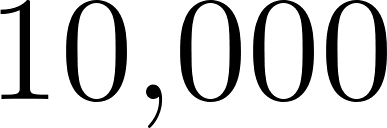, still using a test with 99% sensitivity and 95% specificity. What is 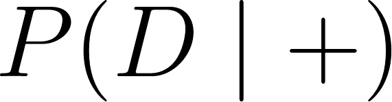now? What lesson does this teach about screening for rare conditions?

Problem 2.7 (Sequential testing). Continuing from the original example (prevalence 1%, sensitivity 99%, specificity 95%), suppose that after the first positive test, the patient is given a second, independent test with the same characteristics, and it also comes back positive. What is the posterior probability of disease now? Hint: use the posterior from the first test as the prior for the second.

Problem 2.8 (Three-hypothesis Bayes). A factory has three machines producing widgets: machine A produces 50% of widgets with a 1% defect rate, machine B produces 30% of widgets with a 2% defect rate, and machine C produces 20% of widgets with a 5% defect rate. A widget is selected at random and found to be defective. What is the probability it came from each machine? Verify that your three posteriors sum to .

Problem 2.9 (Coding exercise). Extend the example program with a function bayes-update that takes a prior probability and a likelihood ratio and returns the posterior probability. Use it to reproduce the medical-screening result. Then apply your function to Problem 2.7 and confirm your answer.