Law of Large Numbers

If you flip a fair coin many times, the fraction of heads gets closer and closer to 1/2. If you roll a fair die many times, the average roll gets closer and closer to 3.5. This is not just an empirical observation. It is a mathematical theorem, and it is one of the pillars of probability theory.

The example program for this chapter is in the file 06_law_of_large_numbers.lisp.

Jakob Bernoulli, in his posthumous Ars Conjectandi (1713), proved the first version of what we now call the Law of Large Numbers for Bernoulli trials. He called his result the “Golden Theorem” and considered it his most important contribution. In modern language, Bernoulli’s theorem says that the sample proportion of successes converges to the true probability as the number of trials grows. Bernoulli was proud enough of his result to spend twenty years polishing it before publication.

The name we use today came later. Siméon Denis Poisson, in 1837, restated and broadened Bernoulli’s result and attached to it the phrase it still carries: la loi des grands nombres, the law of large numbers.

Later refinements by Chebyshev in the nineteenth century, and eventually by Khinchin and Kolmogorov in the twentieth, extended the theorem to arbitrary i.i.d. random variables with finite mean. Chebyshev’s contribution was a simple but powerful inequality (Chapter 3) that gives a proof of the Weak Law of Large Numbers in a few lines. Kolmogorov’s Strong Law is more delicate but rests on the same intuition: averages of many i.i.d. quantities converge to the underlying mean.

Let be independent and identically distributed (i.i.d.) random variables with finite mean 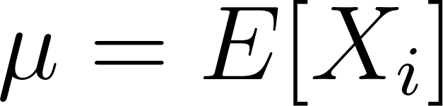. The sample mean after observations is:

By linearity of expectation, 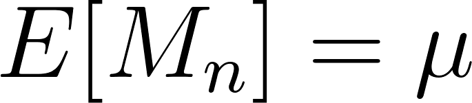for every . The sample mean is always centered on the true mean. But what about its variability?

If the individual variance is 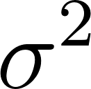, then by additivity of variance for independent variables:

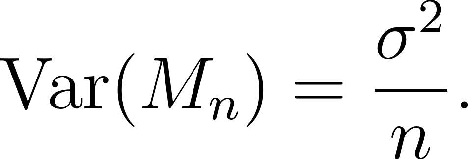
The variance of the sample mean shrinks as grows. Its standard deviation, which is the natural scale for measuring “typical” deviations, shrinks as 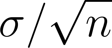. This 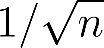rate is fundamental. It says the sample mean concentrates around the true mean, but only slowly: reducing the uncertainty by a factor of 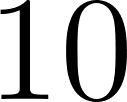requires 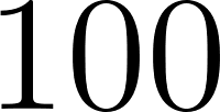times more data.

The Weak Law of Large Numbers states that for any positive number , no matter how small:

In plain language: as the sample size grows, the probability that the sample mean deviates from the true mean by more than any fixed amount shrinks to zero. The sample mean converges in probability to the true mean.

The Weak Law has a beautifully short proof using Chebyshev’s inequality (Chapter 3). Applied to :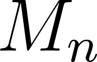

As grows, the right-hand side goes to zero, and so the left-hand side must too. This gives convergence in probability directly. The proof relies only on Chebyshev’s inequality and additivity of variance, both of which are elementary. Bernoulli’s original proof used a much more intricate combinatorial argument; Chebyshev’s cleaner path is the one usually taught today.

The Strong Law of Large Numbers goes further. It states that:

This means that for almost every possible sequence of outcomes, the sample mean eventually settles down to and stays there. The strong law is a stronger statement than the weak law because almost-sure convergence implies convergence in probability but not vice versa.

The difference between the two laws is subtle. The Weak Law says that at each large , the sample mean is probably close to . The Strong Law says that if we watch the whole sequence , the sequence itself converges to with probability . For most practical purposes the two laws give the same guarantee, but the strong law is what the theoretical statistician wants.

Almost-sure statements like the Strong Law are usually proved with a pair of results called the Borel-Cantelli lemmas, which connect the probabilities of a sequence of events to whether infinitely many of them occur. Write 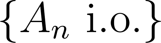for the event that infinitely many of the 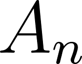happen (“infinitely often”).

The first lemma says that if the probabilities are summable, the events almost surely stop happening:

The second lemma is a partial converse: if the are independent and their probabilities are not summable, then almost surely infinitely many occur:

To see how this powers a strong law, let be the event that the sample mean is far from at step . If we can show 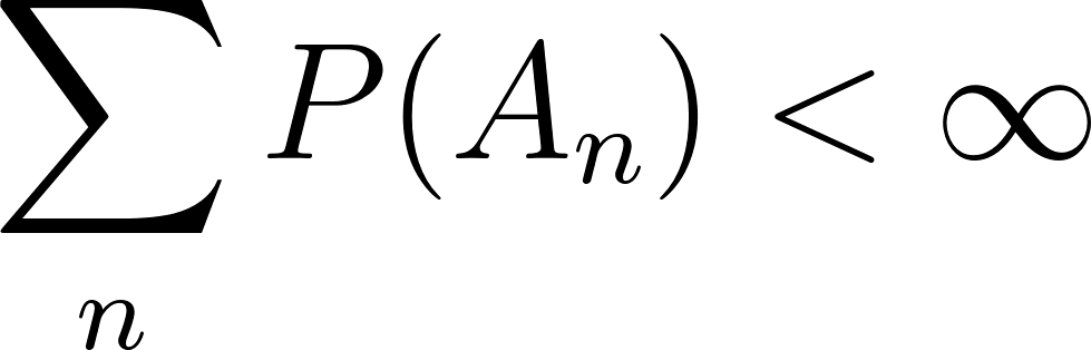, the first lemma says these deviations stop happening for good, which is exactly almost-sure convergence. The Chebyshev bound gives terms of order 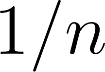, whose sum diverges, so a naive application falls just short. Kolmogorov’s proof closes the gap by working along a cleverly chosen subsequence and controlling the values in between with a maximal inequality. The Borel-Cantelli lemmas are the reason almost-sure convergence can be established at all, and they recur throughout the study of random sequences.

The distinction between weak and strong laws is a special case of a broader theme in probability: different notions of “convergence of random variables.” A brief tour:

• Convergence in probability: for every 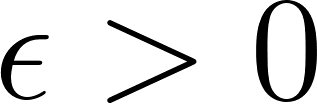, . This is what the Weak Law provides.
• Almost sure convergence: the sequence 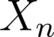converges to 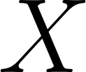pointwise, on all sample paths outside a set of probability zero. This is what the Strong Law provides.
• Convergence in distribution: the CDFs 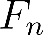converge to 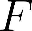at every continuity point of . This is the weakest notion; it is what the Central Limit Theorem in the next chapter provides.
• Convergence in mean square: .

These modes are related by implications: almost sure implies in probability; in probability implies in distribution; mean square implies in probability. Whenever a probability textbook talks about convergence of random variables, it is worth pausing to check which mode is being used.

The Law of Large Numbers requires finite mean. When the mean does not exist, the sample mean does not converge to any deterministic value. The classic pathological example is the Cauchy distribution, which has PDF:

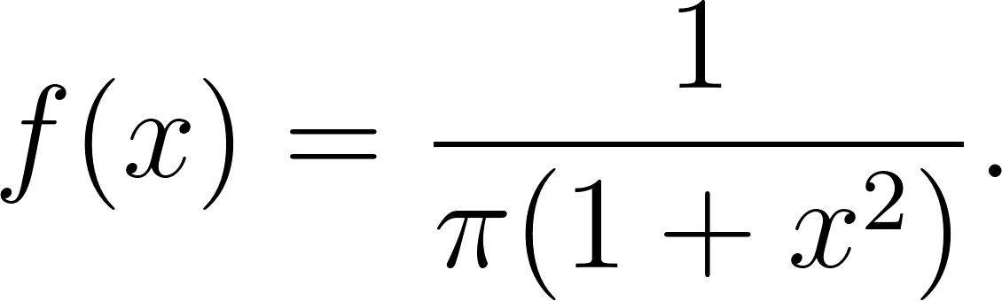
The Cauchy distribution has infinitely heavy tails and no finite mean. Sample means of Cauchy-distributed variables do not settle down; instead, they themselves are Cauchy-distributed. Simulating a million Cauchy draws and averaging them gives an answer that is just as noisy as a single draw. This is a striking counterexample and a reminder that “average enough data” is not a universal solution.

For distributions with finite mean but infinite variance, the Weak Law still holds (in a slightly more delicate form) but the variance-based Chebyshev proof does not apply, and the rate of convergence can be much slower than . Heavy-tailed distributions appear in finance, network traffic, and other real settings where the LLN’s guarantees are still true but weaker than the standard textbook picture suggests.

The Law of Large Numbers is the theoretical justification for using sample averages as estimates of true means. When a pollster surveys 1,000 people and reports that 52% support a candidate, they are relying on the LLN: with a large enough sample, the sample proportion will be close to the true population proportion. When a scientist repeats an experiment many times and averages the results, the LLN guarantees that the average converges to the expected value.

The LLN also explains why casinos always make money in the long run. Each individual bet is random, but over thousands of bets, the average outcome converges to the house edge. The randomness averages out.

The LLN is also the theoretical foundation of Monte Carlo methods (Chapter 8), where we estimate expectations by simulating many samples and averaging them. Every Monte Carlo estimator is a direct application of the LLN.

The program demonstrates the LLN by simulating a fair die and a Bernoulli process, tracking the sample mean as n grows from 10 to 1,000,000:

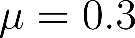
For the fair die, the true mean is . For the Bernoulli process with 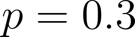, the true mean is .

Watch the column 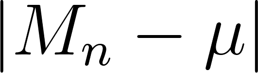shrink as grows. With only rolls, the sample mean can be off by 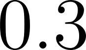or more. By 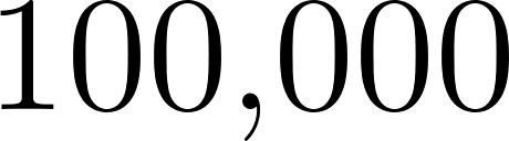rolls, the deviation is typically under 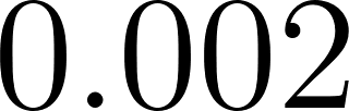. By 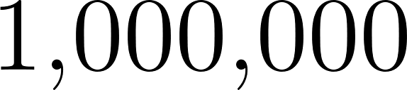, it is essentially zero. This is the Law of Large Numbers in action. The program reseeds its random state on each run, so your exact numbers will differ, but the shrinking trend is always the same.

The convergence is not perfectly monotonic. You can see that the die simulation at has a slightly larger deviation than at . This is expected: the LLN guarantees convergence in the long run, but individual samples can fluctuate. The trend is what matters.

Notice that the deviation shrinks roughly as , not as . Going from to samples reduces the error by about a factor of 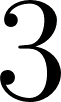(roughly 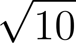), not a factor of . This slow convergence rate is a fundamental limitation of averaging. To halve the error, you need about 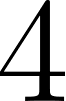times as much data. We will see this rate appear again in the Monte Carlo chapter.

The rate is not a defect of a particular simulation; it is a consequence of the fact that . Standard deviations scale as the square root of variance, so typical deviations of from scale as . This is a universal law for i.i.d. averages with finite variance.

Problem 6.1. For the fair-die simulation, plot (on paper if necessary) the sample mean as a function of . Add a horizontal line at 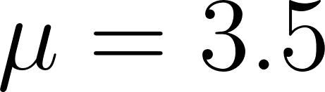and dashed lines at 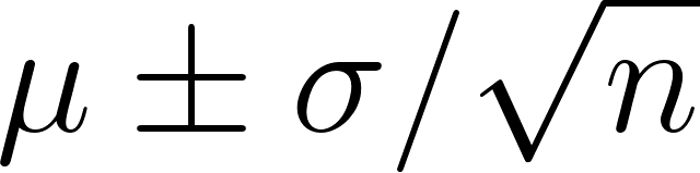using 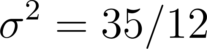. Describe how the sample mean fluctuates relative to those confidence bands.

Problem 6.2 (Chebyshev bound). For a fair die (, ), use Chebyshev’s inequality to bound . Compare against the empirical frequency of this event by running the simulation 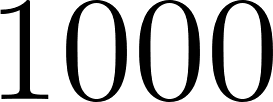times.

Problem 6.3 (Different distributions). Modify the example program to simulate the sample mean of an exponential distribution with rate 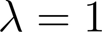. True mean is . Watch the sample mean converge to as grows. Because the exponential is more heavily right-skewed than the fair die, does convergence appear faster or slower?

Problem 6.4 (The Cauchy failure). Add a function that samples from a Cauchy distribution using inverse-CDF: draw 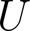from and return . Compute the sample mean for Cauchy samples. Does the sample mean converge, or does it keep jumping around? Explain what you observe in terms of the LLN’s assumption of finite mean.

Problem 6.5 (Empirical variance of M_n). Run independent simulations of a sample mean of die rolls. Record the sample means and compute their variance. Compare against the theoretical prediction .

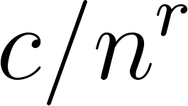
Problem 6.6 (Rate of convergence). For the coin, empirically estimate the rate at which 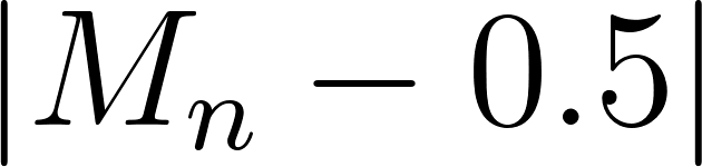shrinks. Fit a curve of the form to the deviations at , and estimate . Does your estimate come out close to 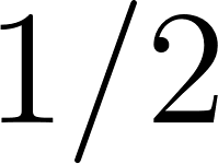as the theory predicts?

Problem 6.7 (Coding exercise). Extend the example program to a function lln-demo that takes a sampling procedure (a thunk returning one sample) and a true mean, and prints a table of the same form as the example’s die output. Test your function on the die, the Bernoulli, and the exponential.

Problem 6.8 (Almost sure vs. in probability). Describe informally what it would look like if the sample mean of a die converged in probability but not almost surely. Would the running sample mean have to keep spiking away from 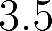forever, or only rarely? Even without a rigorous treatment, this thought experiment sharpens the distinction between the two modes of convergence.