Statistical linear regression models
Watch this video before beginning
Up to this point, we’ve only considered estimation. Estimation is useful, but we also need to know how to extend our estimates to a population. This is the process of statistical inference. Our approach to statistical inference will be through a statistical model. At the bare minimum, we need a few distributional assumptions on the errors. However, we’ll focus on full model assumptions under Gaussianity.
Basic regression model with additive Gaussian errors.
Consider developing a probabilistic model for linear regression. Our starting point will assume a systematic component via a line and then independent and identically distributed Gaussian errors. We can write the model out as:
Here, the \(\epsilon_{i}\) are assumed to be independent and identically distributed as \(N(0, \sigma^2)\). Under this model,
and
This model implies that the \(Y_i\) are independent and normally distributed with means \(\beta_0 + \beta_1 x_i\) and variance \(\sigma^2\). We could write this more compactly as
While this specification of the model is a perhaps better for advanced purposes, specifying the model as linear with additive error terms is generally more useful. With that specification, we can hypothesize and discuss the nature of the errors. In fact, we’ll even cover ways to estimate them to investigate our model assumption.
Remember that our least squares estimates of \(\beta_0\) and \(\beta_1\) are:
It is convenient that under our Gaussian additive error model that the maximum likelihood estimates of \(\beta_0\) and \(\beta_1\) are the least squares estimates.
Interpreting regression coefficients, the intercept
Watch this video before beginning
Our model allows us to attach statistical interpretations to our parameters. Let’s start with the intercept; \(\beta_0\) represents the expected value of the response when the predictor is 0. We can show this as:
Note, the intercept isn’t always of interest. For example, when \(X=0\) is impossible or far outside of the range of data. Take as a specific instance, when X is blood pressure, no one is interested in studying blood pressure’s impact on anything for values near 0.
There is a way to make your intercept more interpretable. Consider that:
Therefore, shifting your \(X\) values by value \(a\) changes the intercept, but not the slope. Often \(a\) is set to \(\bar X\), so that the intercept is interpreted as the expected response at the average \(X\) value.
Interpreting regression coefficients, the slope
Now that we understand how to interpret the intercept, let’s try interpreting the slope. Our slope, \(\beta_1\), is the expected change in response for a 1 unit change in the predictor. We can show that as follows:
Notice that the interpretation of \(\beta_1\) is tied to the units of the X variable. Let’s consider the impact of changing the units.
Therefore, multiplication of \(X\) by a factor \(a\) results in dividing the coefficient by a factor of \(a\).
As an example, suppose that \(X\) is height in meters (m) and \(Y\) is weight in kilograms (kg). Then \(\beta_1\) is kg/m. Converting \(X\) to centimeters implies multiplying \(X\) by 100 cm/m. To get \(\beta_1\) in the right units if we had fit the model in meters, we have to divide by 100 cm/m. Or, we can write out the notation as:
Using regression for prediction
Watch this video before beginning
Regression is quite useful for prediction. If we would like to guess the outcome at a particular value of the predictor, say \(X\), the regression model guesses:
In other words, just find the Y value on the line with the corresponding X value. Regression, especially linear regression, often doesn’t produce the best prediction algorithms. However, it produces parsimonious and interpretable models along with the predictions. Also, as we’ll see later we’ll be able to get easily described estimates of uncertainty associated with our predictions.
Example
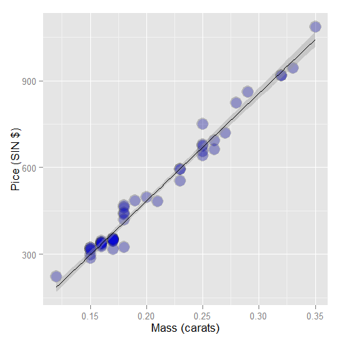
Let’s analyze the diamond data set from the UsingR package.
The data is diamond prices (in Singapore dollars) and diamond weight
in carats. Carats are a standard measure of diamond mass, 0.2 grams.
To get the data use library(UsingR); data(diamond)
First let’s plot the data. Here’s the code I used
library(UsingR)
data(diamond)
library(ggplot2)
g = ggplot(diamond, aes(x = carat, y = price))
g = g + xlab("Mass (carats)")
g = g + ylab("Price (SIN $)")
g = g + geom_point(size = 7, colour = "black", alpha=0.5)
g = g + geom_point(size = 5, colour = "blue", alpha=0.2)
g = g + geom_smooth(method = "lm", colour = "black")
g
and here’s the plot.
First, let’s fit the linear regression model. This is done
with the lm function in R (lm stands for linear model). The
syntax is lm(Y ~ X) where Y is the response and X is the
predictor.
> fit <- lm(price ~ carat, data = diamond)
> coef(fit)
(Intercept)       carat
     -259.6      3721.0
The function coef grabs the fitted coefficients and conveniently names them
for you. Therefore, we estimate an expected 3721.02 (SIN) dollar increase in price
for every carat increase in mass of diamond.
The intercept -259.63 is the expected price of a 0 carat diamond.
We’re not interested in 0 carat diamonds (it’s hard to get a good price for them ;-). Let’s fit the model with a more interpretable intercept by centering our X variable.
> fit2 <- lm(price ~ I(carat - mean(carat)), data = diamond)
coef(fit2)
           (Intercept) I(carat - mean(carat))
                 500.1                 3721.0
Thus the new intercept, 500.1, is the expected price for the average sized diamond of the data (0.2042 carats). Notice the estimated slope didn’t change at all.
Now let’s try changing the scale. This is useful since a one carat increase in a diamond is pretty big. What about changing units to 1/10th of a carat? We can just do this by just dividing the coefficient by 10, no need to refit the model.
Thus, we expect a 372.102 (SIN) dollar change in price for every 1/10th of a carat increase in mass of diamond.
Let’s show via R that this is the same as rescaling our X variable and refitting. To go from 1 carat to 1/10 of a carat units, we need to multiply our data by 10.
> fit3 <- lm(price ~ I(carat * 10), data = diamond)
> coef(fit3)
  (Intercept) I(carat * 10)
       -259.6         372.1
Now, let’s predict the price of a diamond. This should be as easy as just evaluating the fitted line at the price we want to
> newx <- c(0.16, 0.27, 0.34)
> coef(fit)[1] + coef(fit)[2] * newx
[1]  335.7  745.1 1005.5
Therefore, we predict the price to be 335.7, 745.1 and 1005.5 for
a 0.16, 0.26 and 0.34 carat diamond. Of course, our prediction models
will get more elaborate and R has a generic function, predict,
to put our X values into the model for us. The data has to go into
the model as a data frame with the same named X variables.
> predict(fit, newdata = data.frame(carat = newx))
     1      2      3
 335.7  745.1 1005.5
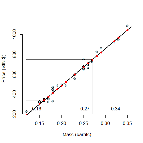
Let’s visualize our prediction. In the following plot, the predicted values at the observed Xs are the red points on the fitted line. The new X values are the at vertical lines, which are connected to the predicted values via the connected horizontal lines.
Exercises
- Fit a linear regression model to the
father.sondataset with the father as the predictor and the son as the outcome. Give a p-value for the slope coefficient and perform the relevant hypothesis test. Watch a video solution. - Refer to question 1. Interpret both parameters. Recenter for the intercept if necessary. Watch a video solution.
- Refer to question 1. Predict the son’s height if the father’s height is 80 inches. Would you recommend this prediction? Why or why not? Watch a video solution.
- Load the
mtcarsdataset. Fit a linear regression with miles per gallon as the outcome and horsepower as the predictor. Interpret your coefficients, recenter for the intercept if necessary. Watch a video solution. - Refer to question 4. Overlay the fit onto a scatterplot. Watch a video solution.
- Refer to question 4. Test the hypothesis of no linear relationship between horsepower and miles per gallon. Watch a video solution.
- Refer to question 4. Predict the miles per gallon for a horsepower of 111. Watch a video solution.