Count data

Watch this video before beginning.

Acknowledgment to Jeff Leek for much of the code and organization of this chapter.

Many data take the form of unbounded count data. For example, consider the number of calls to a call center or the number of flu cases in an area or the number of hits to a web site.

In some of these cases the counts are clearly bounded. However, modeling the counts as unbounded is often done when the upper limit is not known or is very large relative to the number of events.

If the upper bound is known, the techniques we’re discussing can be used to model the proportion or rate. The starting point for most count analysis is the the Poisson distribution.

Poisson distribution

The Poisson distribution is the goto distribution for modeling counts and rates. We’ll define a rate as a count per unit of time. For example your heart rate is often expressed in beats per minute. So, we might look at web hits per day, or disease cases per exposure time (incidence rates). Also, though not exactly a rate, we can treat proportions as if rates when \(n\) is large and the success probability is small.

We would write that a random variable is Poisson, \(X \sim \mathrm{Poisson}(t\lambda)\), if its density function is:

where \(x = 0, 1, \ldots\). The mean of the Poisson is \(E[X] = t\lambda\), thus \(E[X / t] = \lambda\). The variance of the Poisson is \(Var(X) = t\lambda\). The Poisson tends to a normal as \(t\lambda\) gets large and approximates a binomial with large \(n\) and small \(p\) where we would think of \(t\lambda\) as \(n p \).

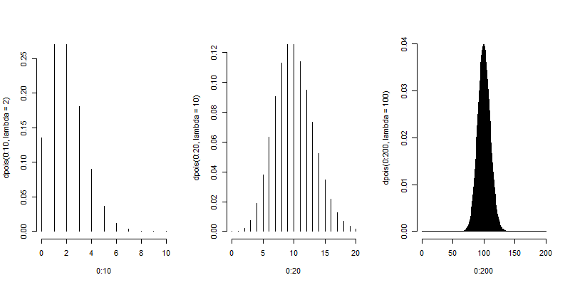
Here are some plots of the Poisson density to illustrate how it closely approximates a normal.

par(mfrow = c(1, 3))
plot(0 : 10, dpois(0 : 10, lambda = 2), type = "h", frame = FALSE)
plot(0 : 20, dpois(0 : 20, lambda = 10), type = "h", frame = FALSE)
plot(0 : 200, dpois(0 : 200, lambda = 100), type = "h", frame = FALSE)

Poisson distribution

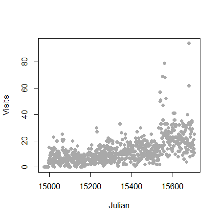
Let’s analyze some data using the Poisson distribution. Consider the daily counts to Jeff Leek’s web site: http://biostat.jhsph.edu/~jleek/

We’re interested in the number of hits per day. Since the unit of time is always one day, set \(t = 1\) and then the Poisson mean is interpreted as web hits per day. If we set \(t = 24\) then our Poisson rate would be interpreted as web hits per hour.

Let’s load the data:

> download.file("https://dl.dropboxusercontent.com/u/7710864/data/gaData.rda",destfi\
le="./data/gaData.rda",method="curl")
> load("./data/gaData.rda")
> gaData$julian = julian(gaData$date)
> head(gaData)
        date visits simplystats julian
1 2011-01-01      0           0  14975
2 2011-01-02      0           0  14976
3 2011-01-03      0           0  14977
4 2011-01-04      0           0  14978
5 2011-01-05      0           0  14979
6 2011-01-06      0           0  14980

> plot(gaData$julian,gaData$visits,pch=19,col="darkgrey",xlab="Julian",ylab="Visits")

Linear regression

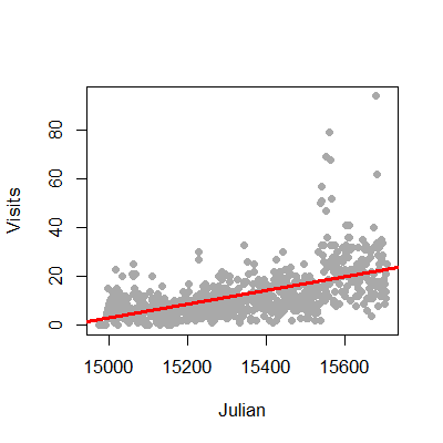
We could try to fit the data with linear regression. This is an often reasonable thing to do. Specifically, we would start with the model

where \(Y_i\) is the number of web hits on day i and \(x_i\) is the day (expressed as a Julian date, the number of days since January 1st, 1970).

This model isn’t anywhere near as objectionable as when applied in the binary case. Two sticking points remain. First, the response is a count and thus is non-negative, while our model doesn’t acknowledge that. Secondly, the errors are typically assumed Gaussian, which is not an accurate approximation for small counts. As the counts get larger, straight application of linear or multivariable regression models becomes more compelling.

1 > plot(gaData$julian,gaData$visits,pch=19,col="darkgrey",xlab="Julian",ylab="Visits")
2 > lm1 = lm(gaData$visits ~ gaData$julian)
3 > abline(lm1,col="red",lwd=3)

The non-negativity could be handled by a (natural) log transformation of the outcome. The log has a special interpretation with respect to regression, so we cover it here. First, there is the issue of zero counts (which can’t be logged). Often a +1 is added to all data before taking the log, a reasonable solution but one that harms the nice interpretation properties of the log. Secondly, a square root or cube root transformation is often applied (which works just fine on zeros). While correcting nicely for skewness, this approach creates the issue of losing the nice interpretation of logs. Thus for the time being, let’s assume no zero counts in the discussion.

Consider now the model:

The quantity \(e^{E[\log(Y)]}\) estimates the geometric mean of \(Y\). When you take the natural log of outcomes and fit a regression model, your exponentiated coefficients estimate things about geometric means. Thus \(e^{\beta_0}\) is the geometric mean of hits on day 0, while \(e^{\beta_1}\) is the relative increase or decrease in hits going from one day to the next.

Let’s try this briefly with Jeff’s data.

> round(exp(coef(lm(I(log(gaData$visits + 1)) ~ gaData$julian))), 5)
  (Intercept) gaData$julian
        0.000         1.002

Thus our model estimates a 0.2% increase in geometric mean daily web hits each day. What’s nice about the geometric mean is it’s a multiplicative quantity. In this case it make sense to think multiplicatively, as we would very naturally think in the terms of percent increases or decreases in the daily rate of web traffic.

Poisson regression

Watch this video before beginning.

Poisson regression is similar to logging the outcome. However, instead we log the model mean exactly as in the binary chapter where we logged the modeled odds. This takes care of the problem of zero counts elegantly.

Consider a model where we assume that \(Y_i \sim \mathrm{Poisson}(\mu_i)\). and

Note that we’re not logging the outcome, we’re logging the assumed mean in the model.

We interpret our coefficients as follows. \(e^\beta_0\) is the expected mean of the outcome when \(x_i = 0\). Using the relationship:

\(e^{\beta_1}\) is the expected relative increase in the outcome for a unit change in the regressor. If there’s more than one regressor in the model, then the coefficients are interpreted in the terms of the other regressors being held fixed.

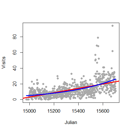
Let’s try it in R for Jeff’s data:

> plot(gaData$julian,gaData$visits,pch=19,col="darkgrey",xlab="Julian",ylab="Visits")
> glm1 = glm(gaData$visits ~ gaData$julian,family="poisson")
> abline(lm1,col="red",lwd=3); lines(gaData$julian,glm1$fitted,col="blue",lwd=3)

Mean-variance relationship

The Poisson model suggest a specific relationship between the mean and the variance. Specifically, if \(Y_i \sim \mathrm{Poisson}(\mu_i)\), then \(E[Y_i] = \mathrm{Var}(Y_i)\). We can often check whether or not this relationship apparently holds. For example, we can plot the fitted values (estimates \(E[Y_i]\)) by generalized version of residuals for Poisson models.

> plot(glm1$fitted,glm1$residuals,pch=19,col="grey",ylab="Residuals",xlab="Fitted")

There are several methods for dealing with data that, while being counts, do not follow the mean variance relationship assumed by the Poisson model. Perhaps the easiest is to assume a so-called quasi-Poisson model. This is from the idea of quasi-likelihood. Here, the model is extended to have the variance be a constant (non-fixed) multiple of the mean. A very related approach are so-called negative binomial models. These models typically assume a more general mean/variance relationship.

Other approaches directly model the mean/variance relationship or rely on asymptotics to be robust to the assumption. We omit a full discussion of general of methods for addressing complex mean variance relationships and simply show a quasi-Poisson fit for the data of this chapter.

> glm2 = glm(visits ~ julian,family="quasipoisson", data = gaData)
#
# Confidence interval expressed as a percentage
> 100 * (exp(confint(glm2)) - 1)[2,]
Waiting for profiling to be done...
                   2.5 %       97.5 %
julian         0.2072924    0.2520376
#
# As compared to the standard Poisson interval
> 100 * (exp(confint(glm1)) - 1)[2,]
Waiting for profiling to be done...
                   2.5 %       97.5 %
julian         0.2192443    0.2399335

In this case the distinction between the intervals is minimal. Again, we reiterate that this only pursues one direction of model departure.

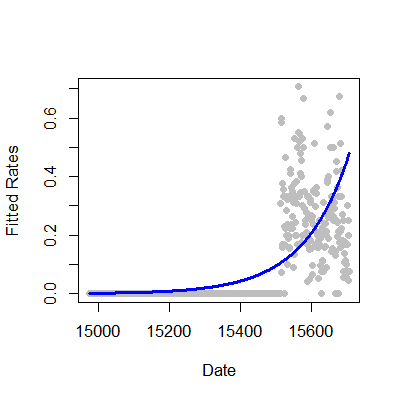
Rates

We fit rates or proportions in Poisson models by including the temporal or sample size component as a (natural) log offset in the model specification. Recall that \(Y_i\) was the number of web hits. Let \(W_i\) be the number of hits directed to the site from the Simply Statistics BLOG site.

Consider the model where

so that

This is a model for the proportion in the sense that \(\mu_i\) is the expected count and our model is:

In this case we were interested in a proportion. If our interest was in rates, counts over a time period, such as incident rate (cases per time at risk), the time variable would be included as the offset.

1 glm3 = glm(simplystats ~ julian(gaData$date),offset=log(visits+1),
2             family="poisson",data=gaData)
3 plot(julian(gaData$date),glm3$fitted,col="blue",pch=19,xlab="Date",ylab="Fitted Coun\
4 ts")
5 points(julian(gaData$date),glm1$fitted,col="red",pch=19)

Exercises

1. Load the dataset Seatbelts as part of the datasets package via data(Seatbelts). Use as.data.frame to convert the object to a dataframe. Fit a Poisson regression GLM with UKDriversKilled as the outcome and kms, PetrolPrice and law as predictors. Interpret your results. Watch a video solution.
2. Refer to question 1. Fit a linear model with the log of drivers killed as the outcome. Interpret your results. Watch a video solution.
3. Refer to question 1. Fit your Poisson log-linear model with drivers as a log offset (to consider the proportion of drivers killed of those killed or seriously injured.) Watch a video solution.
4. Refer to Question 1. Use the anova function to compare models with just law, law and PetrolPrice and all three predictors. Watch a video solution.