Binary GLMs
Watch this video before beginning.
Binary GLMs come from trying to model outcomes that can take only two values. Some examples include: survival or not at the end of a study, winning versus losing of a team and success versus failure of a treatment or product. Often these outcomes are called Bernoulli outcomes, from the Bernoulli distribution named after the famous probabilist and mathematician.
If we happen to have several exchangeable binary outcomes for the same level of covariate values, then that is binomial data and we can aggregate the 0’s and 1’s into the count of 1’s. As an example, imagine if we sprayed insect pests with 4 different pesticides and counted whether they died or not. Then for each spray, we could summarize the data with the count of dead and total number that were sprayed and treat the data as binomial rather than Bernoulli.
Example Baltimore Ravens win/loss
The Baltimore Ravens are an American Football team in the US’s National Football League.2 The data contains the wins and losses of the Ravens by the number of points that they scored. (In American football, the goal is to score more points than your opponent.) It should be clear that there would be a positive relationship between the number of points scored and the probability of winning that particular game.
Let’s load the data and use head to look at the first few rows.
> download.file("https://dl.dropboxusercontent.com/u/7710864/data/ravensData.rda"
              , destfile="./data/ravensData.rda",method="curl")
> load("./data/ravensData.rda")
> head(ravensData)
  ravenWinNum ravenWin ravenScore opponentScore
1           1        W         24             9
2           1        W         38            35
3           1        W         28            13
4           1        W         34            31
5           1        W         44            13
6           0        L         23            24
A linear regression model would look something like this:
Where \(Y_i\) is a binary indicator of whether or not the Ravens won game \(i\)(1 for a win, 0 for a loss). \(X_i\) is the number of points that they scored for that game. and \(\epsilon_i\) is the residual error term.
Under this model then \(\beta_0\) is the expected value of \(Y_i\) given a 0 point game. For a 0/1 variable, the expected value is the probability, so the intercept is the probability that the Ravens win with 0 points scored. Then \(\beta_1\) is the increase in probability of a win for each additional point.
At this point in the book, I hope that fitting and interpreting this model would be second nature.
> lmRavens <- lm(ravensData$ravenWinNum ~ ravensData$ravenScore)
> summary(lmRavens)$coef
                      Estimate Std. Error t value Pr(>|t|)
(Intercept)             0.2850   0.256643   1.111  0.28135
ravensData$ravenScore   0.0159   0.009059   1.755  0.09625
There are numerous problems with this model. First, if the Ravens score more than 63 points in a game, we estimate a 0.0159 * 63, which is greater than 1, increase in the probability of them winning. This is an impossibility, since a probability can’t be greater than 1. Sixty three is an unusual, but not impossible, score in American football, but the principle applies broadly: modeling binary data with linear models results in models that fail the basic assumption of the data.
Perhaps less galling, but still an annoying aspect of the model, is that if the error is assumed to be Gaussian, then our model allows \(Y_i\) to be anything from minus infinity to plus infinity, when we know our data can be only be 0 or 1. If we assume that our errors are discrete to force this, we assume a very strange distribution on the errors.
There also aren’t any transformations to make things better. Any one to one transformation of our outcome is still just going to have two values, thus the same set of problems.
The key insight was to transform the probability of a 1 (win in our example) rather than the data itself. Which transformation is most useful? It turns out that it involves the log of the odds, called the logit.
Odds
You’ve heard of odds before, most likely from discussions of gambling. First note, odds are a fraction greater than 0 but unbounded. The odds are not a percentage or proportion. So, when someone says “The odds are fifty percent”, they are mistaking probability and odds. They likely mean “The probability is fifty percent.”, or equivalently “The odds are one.”, or “The odds are one to one”, or “The odds are fifty [divided by] fifty.” The latter three odds statements are all the same since: 1, 1 / 1 and 50 / 50 are all the same number.
If \(p\) is a probability, the odds are defined as \(o = p/(1-p)\). Note that we can go backwards as \(p = o / (1 + o)\). Thus, if someone says the odds are 1 to 1, they’re saying that the odds are 1 and thus \(p = 1 / (1 + 1) = 0.5\). Conversely, if someone says that the probability that something occurs is 50%, then they mean that \(p=0.5\) so that the odds are \(o = p / (1 - p) = 0.5 / (1 - 0.5) = 1\).
The odds are famously derived using a standard fair game setting. Imagine that you are playing a game where you flip a coin with success probability \(p\) with the following rules:
- If it comes up heads, you win \(X\) dollars.
- If it comes up tails, you lose \(Y\).
What should we set \(X\) and \(Y\) for the game to be fair? Fair means the expected earnings for either player is 0. That is:
This implies \(\frac{Y}{X} = \frac{p}{1 - p} = o\). Consider setting \(X=1\), then \( Y = o\). Thus, the odds can be interpreted as “How much should you be willing to pay for a \(p\) probability of winning a dollar?” If \(p > 0.5\) you have to pay more if you lose than you get if you win. If \(p < 0.5\) you have to pay less if you lose than you get if you win.
So, imagine that I go to a horse race and the odds that a horse loses are 50 to 1. They usually specify in terms of losing at horse tracks, so this would be said to be 50 to 1 “against” where the against is implied and not stated on the boards. The odds of the horse winning are then 1/50. Thus, for a fair bet if I were to bet on the horse winning, they should pay me 50 dollars if he wins and should pay 1 dollar if he loses. (Or any agreed upon multiple, such as 100 dollars if he wins and 2 dollars if he loses.) The implied probability that the horse loses is \(50 / (1 + 50)\).
It’s an interesting side note that the house sets the odds (hence the implied probability) only by the bets coming in. They take a small fee for every bet win or lose (the rake). So, by setting the odds dynamically as the bets roll in, they can guarantee that they make money (risk free) via the rake. Thus the phrase “the house always wins” applies literally. Even more interesting is that by the wisdom of the crowd, the final probabilities tend to match the percentage of times that event happens. That is, house declared 50 to 1 horses tend to win about 1 out of 51 times and lose 50 out of 51 times, even though that 50 to 1 was set by a random collection of mostly uninformed bettors. This is why even your sports junkie friend with seemingly endless up to date sports knowledge can’t make a killing betting on sports; the crowd is just too smart as a group even though most of the individuals know much less.
Finally, and then I’ll get back on track, many of the machine learning algorithms work on this principle of the wisdom of crowds: many small dumb models can make really good models. This is often called ensemble learning, where a lot of independent weak classifiers are combined to make a strong one. Random forests and boosting come to mind as examples. In the Coursera Practical Machine Learning class, we cover ensemble learning algorithms.
Getting back to the issues at hand, recall that probabilities are between 0 and 1. Odds are between 0 and infinity. So, it makes sense to model the log of the odds (the logit), since it goes from minus infinity to plus infinity. The log of the odds is called the logit:
We can go backwards from the logit to the probability with the so-called expit (inverse logit):
Modeling the odds
Let’s come up with notation for modeling the odds. Recall that \(Y_i\) was our outcome, a 0 or 1 indicator of whether or not the Raven’s won game \(i\).
Let
be the probability of a win for number of points \(x_i\). Then the odds that they win is \(p_i / (1 - p_i)\) and the log odds is \(\log{p_i / (1 - p_i)} = \mathrm{logit}(p_i)\).
Logistic regression puts the model on the log of the odds (logit) scale. In other words,
Or, equivalently, we could just say
Interpreting Logistic Regression
Recall our model is:
Let’s write this as:
where \(O(Y_i = 1 ~|~ X_i = x_i)\) refers to the odds. Interpreting \(\beta_0\) is straightforward, it’s the log of the odds of the Ravens winning for a 0 point game. Just like in regular regression, for this to have meaning, a 0 X value has to have meaning. In this case, there’s a structural consideration that’s being ignored in that the Ravens can’t win if they score 0 points (they can only tie or lose). This is an unfortunate assumption of our model.
For interpreting the \(\beta_1\) coefficient, consider the following:
So that \(\beta_1\) is the log of the relative increase in the odds of the Ravens winning for a one point increase in score. The ratio of two odds is called, not surprisingly, the odds ratio. So \(\beta_1\) is the log odds ratio of the Ravens winning associated with a one point increase in score.
We can get rid of the log by exponentiating and then get that \(\exp(\beta_1)\) is the odds ratio associated with a one point increase in score. It’s a nifty fact that you can often perform this exponentiation in your head, since for numbers close to zero, exponentiation is about 1 + that number. So, if you have a logistic regression slope coefficient of 0.01, you know that e to that coefficient is about 1.01. So you know that the coefficient estimates a 1% increase in the odds of a success for every 1 unit increase in the regressor.
Visualizing fitting logistic regression curves
Watch this video before beginning.
Let’s visualize what the logistic regression model is
fitting. Consider setting \(\beta_0\) to 0 and
varying \(\beta_1\) for X being a regressor
equally spaced between -10 and 10. Notice that
the logistic curves vary in their curvature.
= seq(-10, 10, length = 1000)
beta0 = 0; beta1s = seq(.25, 1.5, by = .1)
plot(c(-10, 10), c(0, 1), type = "n", xlab = "X", ylab = "Probability", frame = FALS\
E)
sapply(beta1s, function(beta1) {
y = 1 / (1 + exp( -1 * ( beta0 + beta1 * x ) ))
lines(x, y, type = "l", lwd = 3)
}
)
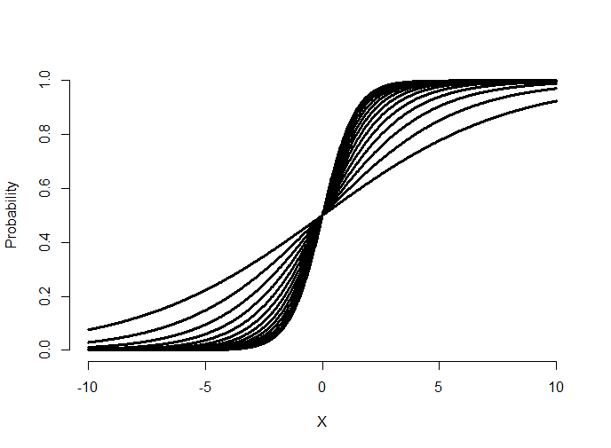
Try making the slope negative and see what happens. (It flips the curve from increasing to decreasing.) Now let’s hold \(\beta_1\) fixed and vary \(\beta_0\).
= seq(-10, 10, length = 1000)
beta0s = seq(-2, 2, by = .5); beta1 = 1
plot(c(-10, 10), c(0, 1), type = "n", xlab = "X", ylab = "Probability", frame = FALS\
E)
sapply(beta0s, function(beta0) {
y = 1 / (1 + exp( -1 * ( beta0 + beta1 * x ) ))
lines(x, y, type = "l", lwd = 3)
}
)
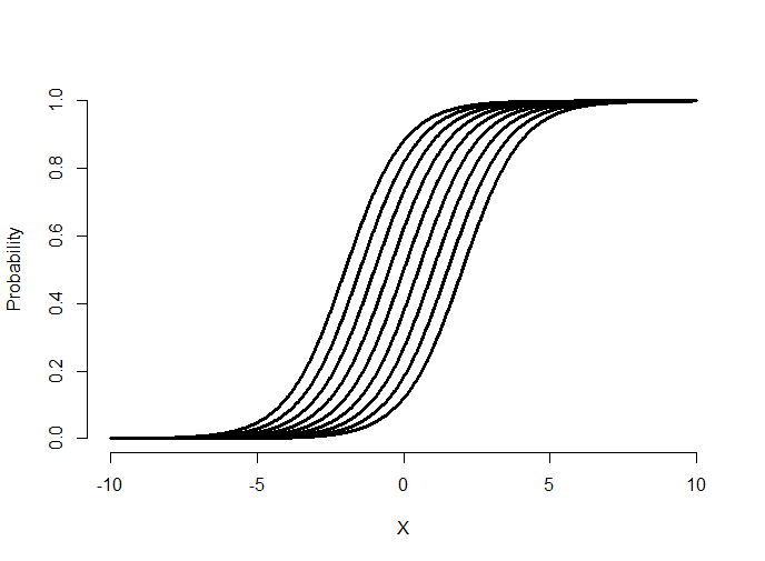
Notice that varying the intercept shifts the curve back and forth. Let’s superimpose some data with the fitted curve.
= seq(-10, 10, length = 1000)
beta0 = 0; beta1 = 1
p = 1 / (1 + exp(-1 * (beta0 + beta1 * x)))
y = rbinom(prob = p, size = 1, n = length(p))
plot(x, y, frame = FALSE, xlab = "x", ylab = "y")
lines(lowess(x, y), type = "l", col = "blue", lwd = 3)
fit = glm(y ~ x, family = binomial)
lines(x, predict(fit, type = "response"), lwd = 3, col = "red")
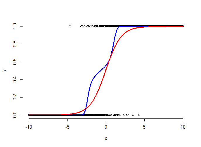
The plot above shows the simulated binary data (black points), the fitted logistic curve (red) and a lowess smoother through the data (blue). The lowess smoother shows a non-parametric estimate of the probability of a success at each x value. Think of it as a moving proportion. Logistic regression gets to move around the intercept and slope of the logistic curve to fit the data well. Here the fit says that the probability of a 1 for low values of x is very small, the probability of a 1 for high values of x is high and it is intermediate at the points in the middle.
Ravens logistic regression
Watch this video before beginning.
Now let’s run our binary regression model on the Ravens data.
> logRegRavens = glm(ravensData$ravenWinNum ~ ravensData$ravenScore,family="binomial\")
> summary(logRegRavens)
Call:
glm(formula = ravensData$ravenWinNum ~ ravensData$ravenScore,
family = "binomial")
Deviance Residuals:
Min 1Q Median 3Q Max
-1.758 -1.100 0.530 0.806 1.495
Coefficients:
Estimate Std. Error z value Pr(>|z|)
(Intercept) -1.6800 1.5541 -1.08 0.28
ravensData$ravenScore 0.1066 0.0667 1.60 0.11
(Dispersion parameter for binomial family taken to be 1)
Null deviance: 24.435 on 19 degrees of freedom
Residual deviance: 20.895 on 18 degrees of freedom
AIC: 24.89
Number of Fisher Scoring iterations: 5
## plotting the fit
> plot(ravensData$ravenScore,logRegRavens$fitted,pch=19,col="blue",xlab="Score",ylab\
="Prob Ravens Win")
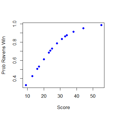
In this case, the data only covers some of the logistic curve, so that the full “S” of the curve isn’t visible. To interpret our coefficients, let’s exponentiate them.
> exp(logRegRavens$coeff)
          (Intercept) ravensData$ravenScore
               0.1864                1.1125
> exp(confint(logRegRavens))
                         2.5 % 97.5 %
(Intercept)           0.005675  3.106
ravensData$ravenScore 0.996230  1.303
The first line of code shows that the exponentiated slope coefficient is 1.11. Thus, we estimate a 11% increase in the odds of winning per 1 point increase in score. However, the data are variable and the confident interval goes from 0.99 to 1.303. Since this interval contains 1 (or contains 0 on the log scale), it’s not statistically significant. (It’s pretty close, though.)
If we had included another variable in our model, say home versus away game indicator, then our slope is interpreted holding the value of the covariate held fixed. Just like in multivariable regression.
We can also compare nested models using ANOVA and, by and large, our general model discussion carries over to this setting as well.
Some summarizing comments
Odds aren’t probabilities. In binary GLMs, we model the log of the odds (logit) and our slope parameters are interpreted as log odds ratios. Odds ratios of 1 or log odds ratios of 0 are interpreted as no effect of the regressor on the outcome.
Exercises
- Load the dataset
Seatbeltsas part of thedatasetspackage viadata(Seatbelts). Useas.data.frameto convert the object to a dataframe. Create a new outcome variable for whether or not greater than 119 drivers were killed that month. Fit a logistic regression GLM with this variable as the outcome andkms,PetrolPriceandlawas predictors. Interpret your parameters. Watch a video solution. - Fit a binomial model with
DriversKilledas the outcome anddriversas the total count withkms,PetrolPriceandlawas predictors, interpret your results. Watch a video solution. - Refer to Question 1. Use the
anovafunction to compare models with justlaw,lawandPetrolPriceand all three predictors. Watch a video solution.