Residuals

Watch this video before beginning

Residual variation

Residuals represent variation left unexplained by our model. We emphasize the difference between residuals and errors. The errors are the unobservable true deviations from the known coefficients, while residuals are the observable deviations from the estimated coefficients. In a sense, the residuals are estimates of the errors.

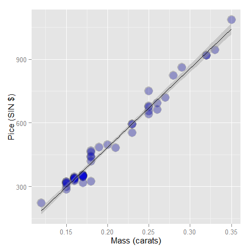
Consider again the diamond data set from UsingR. Recall that the data is diamond prices (Singapore dollars) and diamond weight in carats (standard measure of diamond mass, 0.2g). To get the data use library(UsingR); data(diamond). Recall that the data and our linear regression fit looked like the following:

Recall our linear model was

where we are assuming that \(\epsilon_i \sim N(0, \sigma^2)\). Our observed outcome is \(Y_i\) with associated predictor value, \(X_i\). Let’s label the predicted outcome for index \(i\) as \(\hat Y_i\). Recall that we obtain our predictions by plugging our observed \(X_i\) into the linear regression equation:

The residual is defined as the difference the between the observed and predicted outcome

The residuals are exactly the vertical distance between the observed data point and the associated point on the regression line. Positive residuals have associated Y values above the fitted line and negative residuals have values below.

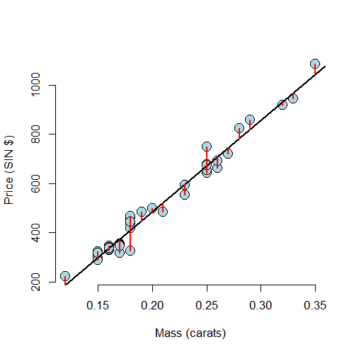
Least squares minimizes the sum of the squared residuals, \(\sum_{i=1}^n e_i^2\). Note that the \(e_i\) are observable, while the errors, \(\epsilon_i\) are not. The residuals can be thought of as estimates of the errors.

Properties of the residuals

Let’s consider some properties of the residuals. First, under our model, their expected value is 0, \(E[e_i] = 0\). If an intercept is included, \(\sum_{i=1}^n e_i = 0\). Note this tells us that the residuals are not independent. If we know \(n-1\) of them, we know the \(n^{th}\). In fact, we will only have \(n-p\) free residuals, where \(p\) is the number of coefficients in our regression model, so \(p=2\) for linear regression with an intercept and slope. If a regressor variable, \(X_i\), is included in the model then \(\sum_{i=1}^n e_i X_i = 0\).

What do we use residuals for? Most importantly, residuals are useful for investigating poor model fit. Residual plots highlight poor model fit.

Another use for residuals is to create covariate adjusted variables. Specifically, residuals can be thought of as the outcome (Y) with the linear association of the predictor (X) removed. So, for example, if you wanted to create a weight variable with the linear effect of height removed, you would fit a linear regression with weight as the outcome and height as the predictor and take the residuals. (Note this only works if the relationship is linear.)

Finally, we should note the different sorts of variation one encounters in regression. There’s the total variability in our response, usually called total variation. One then differentiates residual variation (variation after removing the predictor) from systematic variation (variation explained by the regression model). These two kinds of variation add up to the total variation, which we’ll see later.

Example

Watch this video before beginning

The code below shows how to obtain the residuals.

> data(diamond)
> y <- diamond$price; x <- diamond$carat; n <- length(y)
> fit <- lm(y ~ x)
## The easiest way to get the residuals
> e <- resid(fit)
## Obtain the residuals manually, get the predicted Ys first
> yhat <- predict(fit)
## The residuals are y - yhat. Let's check by comparing this
## with R's build in resid function
> max(abs(e -(y - yhat)))
[1] 9.486e-13
## Let's do it again hard coding the calculation of Yhat
max(abs(e - (y - coef(fit)[1] - coef(fit)[2] * x)))
[1] 9.486e-13

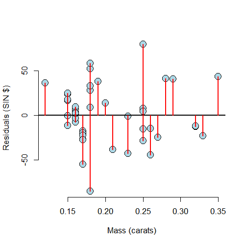
Residuals versus X

A useful plot is the residuals versus the X values. This allows us to zoom in on instances of poor model fit. Whenever we look at a residual plot, we are searching for systematic patterns of any sort. Here’s the plot for diamond data.

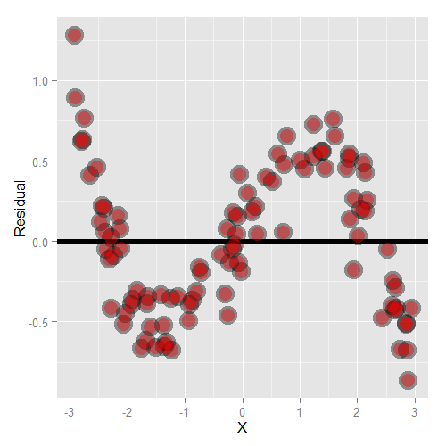
Let’s go through some contrived examples to highlight. Here’s a plot of nonlinear data where we’ve fit a line.

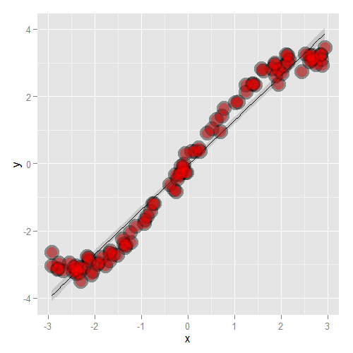
Here’s what happens when you focus in on the residuals.

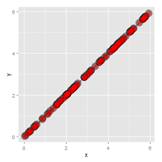
Another common feature where our model fails is when the variance around the regression line is not constant. Remember our errors are assumed to be Gaussian with a constant error. Here’s an example where heteroskedasticity is not at all apparent in the scatterplot.

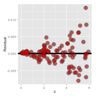
Now look at the consequences of focusing in on the residuals.

If we look at the residual plot for the diamond data, things don’t look so bad.

Estimating residual variation

Watch this before beginning

We’ve talked at length about how to estimate \(\beta_0\) and \(\beta_1\). However, there’s another parameter in our model, \(\sigma\). Recall that our model is \(Y_i = \beta_0 + \beta_1 X_i + \epsilon_i\), where \(\epsilon_i \sim N(0, \sigma^2)\).

It seems natural to use our residual variation to estimate population error variation. In fact, the maximum likelihood estimate of \(\sigma^2\) is \(\frac{1}{n}\sum_{i=1}^n e_i^2\), the average squared residual. Since the residuals have a zero mean (if an intercept is included), this is close to the the calculating the variance of the residuals. However, to obtain unbiasedness, most people use

The \(n-2\) instead of \(n\) is so that \(E[\hat \sigma^2] = \sigma^2\). This is exactly analogous to dividing by \(n-1\) in the ordinary variance calculation. In fact, the ordinary variance (using var in R on a vector) is exactly the same as the residual variance estimate from a model that has an intercept and no slope. The \(n-2\) instead of \(n-1\) when we include a slope can be thought of as losing a degree of freedom from having to estimate an extra parameter (the slope).

Most of this is typically opaque to the user, since we just grab the correct residual variance output from lm. But, to solidify the concepts, let’s go through the diamond example to make sure that we can hard code the estimates on our own. (And from then on we’ll just use lm.)

Diamond example

> y <- diamond$price; x <- diamond$carat; n <- length(y)
> fit <- lm(y ~ x)
## the estimate from lm
> summary(fit)$sigma
[1] 31.84
## directly calculating from the residuals
> sqrt(sum(resid(fit)^2) / (n - 2))
[1] 31.84

Summarizing variation

A way to think about regression is in the decomposition of variability of our response. The total variability in our response is the variability around an intercept. This is also the variance estimate from a model with only an intercept:

The regression variability is the variability that is explained by adding the predictor. Mathematically, this is:

\(\mbox{Regression variability} = \sum_{i=1}^n (\hat Y_i - \bar Y)^2\).

The residual variability is what’s leftover around the regression line

It’s a nice fact that the error and regression variability add up to the total variability:

Thus, we can think of regression as explaining away variability. The fact that all of the quantities are positive and that they add up this way allows us to define the proportion of the total variability explained by the model.

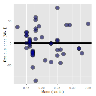
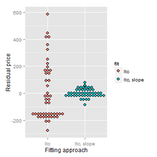
Consider our diamond example again. The plot below shows the variation explained by a model with an intercept only (representing total variation) and then the mass is included as a linear predictor. Notice how much the variation decreases when including the diamond mass.

Here’s the code:

e = c(resid(lm(price ~ 1, data = diamond)),
      resid(lm(price ~ carat, data = diamond)))
fit = factor(c(rep("Itc", nrow(diamond)),
               rep("Itc, slope", nrow(diamond))))
g = ggplot(data.frame(e = e, fit = fit), aes(y = e, x = fit, fill = fit))
g = g + geom_dotplot(binaxis = "y", size = 2, stackdir = "center", binwidth = 20)
g = g + xlab("Fitting approach")
g = g + ylab("Residual price")
g

R squared

R squared is the percentage of the total variability that is explained by the linear relationship with the predictor

Here are some summary notes about R squared.

• \(R^2\) is the percentage of variation explained by the regression model.
• $$ 0 \leq R^2 \leq 1 $$
• \(R^2\) is the sample correlation squared
• \(R^2\) can be a misleading summary of model fit.
  • Deleting data can inflate it.
  • (For later.) Adding terms to a regression model always increases \(R^2\).

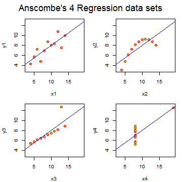
Anscombe’s residuals (named after their inventor) are a famous example of how R squared doesn’t tell the whole story about model fit. In this example, four data sets have equivalent R squared values and beta values, but dramatically different model fits. The result is to suggest that reducing data to a single number, be it R squared, a test statistic or a P-value, often masks important aspects of the data. The code is quite simple: data(anscombe);example(anscombe).

Exercises

1. Fit a linear regression model to the father.son dataset with the father as the predictor and the son as the outcome. Plot the father’s height (horizontal axis) versus the residuals (vertical axis). Watch a video solution.
2. Refer to question 1. Directly estimate the residual variance and compare this estimate to the output of lm. Watch a video solution.
3. Refer to question 1. Give the R squared for this model. Watch a video solution.
4. Load the mtcars dataset. Fit a linear regression with miles per gallon as the outcome and horsepower as the predictor. Plot horsepower versus the residuals. Watch a video solution.
5. Refer to question 4. Directly estimate the residual variance and compare this estimate to the output of lm. Watch a video solution.
6. Refer to question 4. Give the R squared for this model. Watch a video solution.