Regression inference
In this chapter, we’ll consider statistical inference for regression models.
Reminder of the model
Consider our regression model:
where \(\epsilon \sim N(0, \sigma^2)\). Let’s consider some ways for doing inference for our regression parameters. For this development, we assume that the true model is known. We also assume that you’ve seen confidence intervals and hypothesis tests before. If not, consider taking the Statistical Inference course and reading the accompanying book before approaching this material.
Remember our estimates:
and
Review
Let’s review some important components of statistical inference. Consider statistics like the following:
where \(\hat \theta \) is an estimate of interest, \(\theta\) is the estimand of interest and \( \hat \sigma_{\hat \theta} \) is the standard error of \(\hat \theta\). We see that in many cases such statistics often have the following properties:
- They are normally distributed and have a finite sample Student’s T distribution under normality assumptions.
- They can be used to test \(H_0 : \theta = \theta_0\) versus \(H_a : \theta >,
- They can be used to create a confidence interval for \(\theta\) via \(\hat \theta \pm Q_{1-\alpha/2} \hat \sigma_{\hat \theta}\) where \(Q_{1-\alpha/2}\) is the relevant quantile from either a normal or T distribution.
In the case of regression with iid Gaussian sampling assumptions on the errors, our inferences will follow very similarly to what you saw in your inference class.
We won’t cover asymptotics for regression analysis, but suffice it to say that under assumptions on the ways in which the \(X\) values are collected, the iid sampling model and mean model, the normal results hold to create intervals and confidence intervals
Results for the regression parameters
First, we need standard errors for our regression parameters. These are given by:
and
In practice, \(\sigma^2\) is replaced by its residual variance estimate covered in the last chapter.
Given how often this came up in inference, it’s probably not surprising that under iid Gaussian errors
follows a t distribution with n-2 degrees of freedom and a normal distribution for large n. This can be used to create confidence intervals and perform hypothesis tests.
Example diamond data set
Let’s go through a didactic example using our diamond pricing data.
First, let’s define our outcome, predictor and estimate all of the parameters.
(Note, again we’re hard coding these results, but lm will give it to us automatically).
library(UsingR); data(diamond)
y <- diamond$price; x <- diamond$carat; n <- length(y)
beta1 <- cor(y, x) * sd(y) / sd(x)
beta0 <- mean(y) - beta1 * mean(x)
e <- y - beta0 - beta1 * x
sigma <- sqrt(sum(e^2) / (n-2))
ssx <- sum((x - mean(x))^2)
Now let’s calculate the standard errors for our regression coefficients and the t statistic. The natural null hypotheses are \(H_0: \beta_j = 0\). So our t statistics are just the estimates divided by their standard errors.
<- (1 / n + mean(x) ^ 2 / ssx) ^ .5 * sigma
seBeta1 <- sigma / sqrt(ssx)
tBeta0 <- beta0 / seBeta0
tBeta1 <- beta1 / seBeta1
Now let’s consider getting P-values. Recall that P-values are the probability
of getting a statistic as or larger than was actually obtained, where the
probability is calculated under the null hypothesis. Below I also do some
formatting to get it to look like the output from lm.
> pBeta0 <- 2 * pt(abs(tBeta0), df = n - 2, lower.tail = FALSE)
> pBeta1 <- 2 * pt(abs(tBeta1), df = n - 2, lower.tail = FALSE)
> coefTable <- rbind(c(beta0, seBeta0, tBeta0, pBeta0), c(beta1, seBeta1, tBeta1, pB\
eta1))
> colnames(coefTable) <- c("Estimate", "Std. Error", "t value", "P(>|t|)")
> rownames(coefTable) <- c("(Intercept)", "x")
> coefTable
            Estimate Std. Error t value   P(>|t|)
(Intercept)   -259.6      17.32  -14.99 2.523e-19
x             3721.0      81.79   45.50 6.751e-40
The first column is the actual estimates. The second is the standard
errors, the third is the t value (the first divided by the second) and the
final is the t probability of getting an unsigned statistic that large under
the null hypothesis (the P-value for the two sided test).
Of course, we don’t actually go through this exercise every time; lm does
it for us.
> fit <- lm(y ~ x);
> summary(fit)$coefficients
            Estimate Std. Error t value  Pr(>|t|)
(Intercept)   -259.6      17.32  -14.99 2.523e-19
x             3721.0      81.79   45.50 6.751e-40
Remember, we reject if our P-value is less than our desired type I error rate. In both cases the test is for whether or not the parameter is zero. This is almost always of interest for the slope, but frequently a zero intercept isn’t of interest so that P-value is often disregarded.
For the slope, a value of zero represents no linear relationship between the predictor and response. So, the P-value is for performing a test of whether any (linear) relationship exist or not.
Getting a confidence interval
Recall from your inference class, a fair number of confidence intervals take the form of an estimate plus or minus a t quantile times a standard error. Let’s use that formula to create confidence intervals for our regression parameters. Let’s first do the intercept.
> sumCoef <- summary(fit)$coefficients
> sumCoef[1,1] + c(-1, 1) * qt(.975, df = fit$df) * sumCoef[1, 2]
[1] -294.5 -224.8
Now let’s do the slope:
> (sumCoef[2,1] + c(-1, 1) * qt(.975, df = fit$df) * sumCoef[2, 2]) / 10
[1] 355.6 388.6
So, we would interpret this as: “with 95% confidence, we estimate that a 0.1 carat increase in diamond size results in a 355.6 to 388.6 increase in price in (Singapore) dollars”.
Prediction of outcomes
Finally, let’s consider prediction again. Consider the problem of predicting Y at a value of X. In our example, this is predicting the price of a diamond given the carat.
We’ve already covered that the estimate for prediction at point \(x_0\) is:
A standard error is needed to create a prediction interval. This is important, since predictions by themselves don’t convey anything about how accurate we would expect the prediction to be. Take our diamond example. Because the model fits so well, we would be surprised if we tried to sell a diamond and the offers were well off our model prediction (since it seems to fit quite well).
There’s a subtle, but important, distinction between intervals for the regression line at point \(x_0\) and the prediction of what a \(y\) would be at point \(x_0\). What differs is the standard error:
For the line at \(x_0\) the standard error is,
For the prediction interval at \(x_0\) the standard error is
Notice that the prediction interval standard error is a little larger than the error for a line. Think of it this way. If we want to predict a Y value at a particular X value, and we knew the actual true slope and intercept, there would still be error. However, if we only wanted to predict the value at the line at that X value, there would be no variance, since we already know the line.
Thus, the variation for the line only considers how hard it is to estimate the regression line at that X value. The prediction interval includes that variation, as well as the extra variation unexplained by the relationship between Y and X. So, it has to be a little wider.
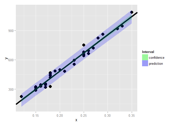
For the diamond example, here’s both the mean value and prediction interval.
(code and plot). Notice that to get the various intervals, one has to
use one of the options interval="confidence" or interval="prediction" in the
prediction function.
library(ggplot2)
newx = data.frame(x = seq(min(x), max(x), length = 100))
p1 = data.frame(predict(fit, newdata= newx,interval = ("confidence")))
p2 = data.frame(predict(fit, newdata = newx,interval = ("prediction")))
p1$interval = "confidence"
p2$interval = "prediction"
p1$x = newx$x
p2$x = newx$x
dat = rbind(p1, p2)
names(dat)[1] = "y"
g = ggplot(dat, aes(x = x, y = y))
g = g + geom_ribbon(aes(ymin = lwr, ymax = upr, fill = interval), alpha = 0.2)
g = g + geom_line()
g = g + geom_point(data = data.frame(x = x, y=y), aes(x = x, y = y), size = 4)
g
Summary notes
- Both intervals have varying widths.
- Least width at the mean of the Xs.
- We are quite confident in the regression line, so that
interval is very narrow.
- If we knew \(\beta_0\) and \(\beta_1\) this interval would have zero width.
- The prediction interval must incorporate the variability
in the data around the line.
- Even if we knew \(\beta_0\) and \(\beta_1\) this interval would still have width. *
Exercises
- Test whether the slope coefficient for the
father.sondata is different from zero (father as predictor, son as outcome). Watch a video solution. - Refer to question 1. Form a confidence interval for the slope coefficient. Watch a video solution
- Refer to question 1. Form a confidence interval for the intercept (center the fathers’ heights first to get an intercept that is easier to interpret). Watch a video solution.
- Refer to question 1. Form a mean value interval for the expected son’s height at the average father’s height. Watch a video solution.
- Refer to question 1. Form a prediction interval for the son’s height at the average father’s height. Watch a video solution.
- Load the mtcars dataset. Fit a linear regression with miles per gallon as the outcome and horsepower as the predictor. Test whether or not the horsepower power coefficient is statistically different from zero. Interpret your test.
- Refer to question 6. Form a confidence interval for the slope coefficient.
- Refer to question 6. Form a confidence interval for the intercept (center the HP variable first).
- Refer to question 6. Form a mean value interval for the expected MPG for the average HP.
- Refer to question 6. Form a prediction interval for the expected MPG for the average HP.
- Refer to question 6. Create a plot that has the fitted regression line plus curves at the expected value and prediction intervals.