Ordinary least squares

Watch this video before beginning

Ordinary least squares (OLS) is the workhorse of statistics. It gives a way of taking complicated outcomes and explaining behavior (such as trends) using linearity. The simplest application of OLS is fitting a line.

General least squares for linear equations

Consider again the parent and child height data from Galton.

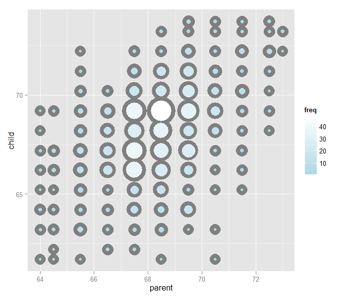
Let’s try fitting the best line. Let \(Y_i\) be the \(i^{th}\) child’s height and \(X_i\) be the \(i^{th}\) (average over the pair of) parental heights. Consider finding the best line of the form

Let’s try using least squares by minimizing the following equation over \(\beta_0\) and \(\beta_1\):

Minimizing this equation will minimize the sum of the squared distances between the fitted line at the parents’ heights (\( \beta_1 X_i\)) and the observed child heights (\(Y_i\)).

The result actually has a closed form. Specifically, the least squares of the line:

through the data pairs \((X_i, Y_i)\) with \(Y_i\) as the outcome obtains the line \(Y = \hat \beta_0 + \hat \beta_1 X\) where:

At this point, a couple of notes are in order. First, the slope, \(\hat \beta_1\), has the units of \(Y / X\). Secondly, the intercept, \(\hat \beta_0\), has the units of \(Y\).

The line passes through the point \((\bar X, \bar Y)\). If you center your Xs and Ys first, then the line will pass through the origin. Moreover, the slope is the same one you would get if you centered the data, \((X_i - \bar X, Y_i - \bar Y)\), and either fit a linear regression or regression through the origin.

To elaborate, regression through the origin, assuming that \(\beta_0 = 0\), yields the following solution to the least squares criteria:

This is exactly the correlation times the ratio in the standard deviations if the both the Xs and Ys have been centered first. (Try it out using R to verify this!)

It is interesting to think about what happens when you reverse the role of \(X\) and \(Y\). Specifically, the slope of the regression line with \(X\) as the outcome and \(Y\) as the predictor is \(Cor(Y, X) Sd(X)/ Sd(Y)\).

If you normalized the data, \(\{ \frac{X_i - \bar X}{Sd(X)}, \frac{Y_i - \bar Y}{Sd(Y)}\}\), the slope is simply the correlation, \(Cor(Y, X)\), regardless of which variable is treated as the outcome.

Revisiting Galton’s data

Watch this video before beginning

Let’s double check our calculations using R

> y <- galton$child
> x <- galton$parent
> beta1 <- cor(y, x) *  sd(y) / sd(x)
> beta0 <- mean(y) - beta1 * mean(x)
> rbind(c(beta0, beta1), coef(lm(y ~ x)))
     (Intercept)      x
[1,]       23.94 0.6463
[2,]       23.94 0.6463

We can see that the result of lm is identical to hard coding the fit ourselves. Let’s reverse the outcome/predictor relationship.

> beta1 <- cor(y, x) *  sd(x) / sd(y)
> beta0 <- mean(x) - beta1 * mean(y)
> rbind(c(beta0, beta1), coef(lm(x ~ y)))
     (Intercept)      y
[1,]       46.14 0.3256
[2,]       46.14 0.3256

Now let’s show that regression through the origin yields an equivalent slope if you center the data first

> yc <- y - mean(y)
> xc <- x - mean(x)
> beta1 <- sum(yc * xc) / sum(xc ^ 2)
c(beta1, coef(lm(y ~ x))[2])
            x
0.6463 0.6463

Now let’s show that normalizing variables results in the slope being the correlation.

> yn <- (y - mean(y))/sd(y)
> xn <- (x - mean(x))/sd(x)
> c(cor(y, x), cor(yn, xn), coef(lm(yn ~ xn))[2])
                  xn
0.4588 0.4588 0.4588

The image below plots the data again, the best fitting line and standard error bars for the fit. We’ll work up to that point later. But, understanding that our fitted line is estimated with error is an important concept. You can find the code for the plot here.

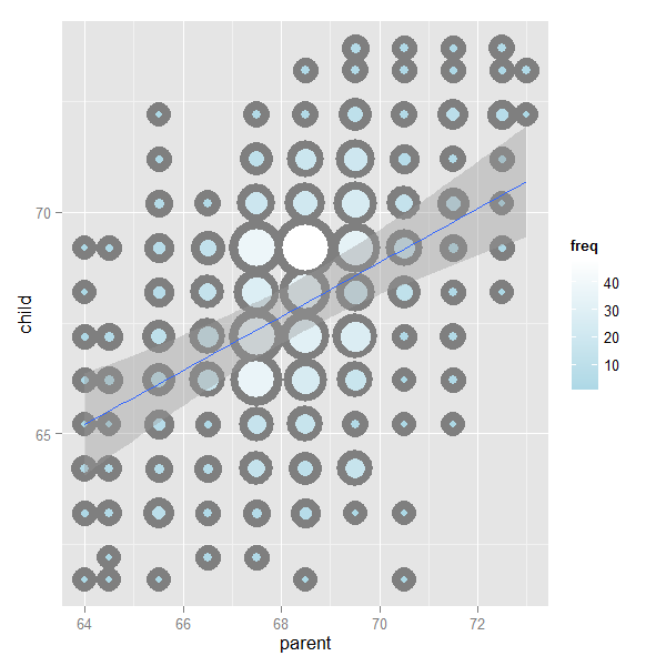
Showing the OLS result

If you would like to see a proof of why the ordinary least squares result works out to be the way that it is: watch this video.

Exercises

1. Install and load the package UsingR and load the father.son data with data(father.son). Get the linear regression fit where the son’s height is the outcome and the father’s height is the predictor. Give the intercept and the slope, plot the data and overlay the fitted regression line. Watch a video solution.
2. Refer to problem 1. Center the father and son variables and refit the model omitting the intercept. Verify that the slope estimate is the same as the linear regression fit from problem 1. Watch a video solution.
3. Refer to problem 1. Normalize the father and son data and see that the fitted slope is the correlation. Watch a video solution.
4. Go back to the linear regression line from Problem 1. If a father’s height was 63 inches, what would you predict the son’s height to be? Watch a video solution.
5. Consider a data set where the standard deviation of the outcome variable is double that of the predictor. Also, the variables have a correlation of 0.3. If you fit a linear regression model, what would be the estimate of the slope? Watch a video solution.
6. Consider the previous problem. The outcome variable has a mean of 1 and the predictor has a mean of 0.5. What would be the intercept? Watch a video solution.
7. True or false, if the predictor variable has mean 0, the estimated intercept from linear regression will be the mean of the outcome? Watch a video solution.
8. Consider problem 5 again. What would be the estimated slope if the predictor and outcome were reversed? Watch a video solution.