Regression to the mean

Watch this video before beginning

A historically famous idea, regression to the mean

Here is a fundamental question. Why is it that the children of tall parents tend to be tall, but not as tall as their parents? Why do children of short parents tend to be short, but not as short as their parents? Conversely, why do parents of very short children, tend to be short, but not a short as their child? And the same with parents of very tall children?

We can try this with anything that is measured with error. Why do the best performing athletes this year tend to do a little worse the following? Why do the best performers on hard exams always do a little worse on the next hard exam?

These phenomena are all examples of so-called regression to the mean. Regression to the mean, was invented by Francis Galton in the paper “Regression towards mediocrity in hereditary stature” The Journal of the Anthropological Institute of Great Britain and Ireland , Vol. 15, (1886). The idea served as a foundation for the discovery of linear regression.

Think of it this way, imagine if you simulated pairs of random normals. The largest first ones would be the largest by chance, and the probability that there are smaller for the second simulation is high. In other words \(P(Y < x | X = x)\) gets bigger as \(x\) heads to the very large values. Similarly \(P(Y > x | X = x)\) gets bigger as \(x\) heads to very small values. Think of the regression line as the intrinsic part and the regression to the mean as the result of noise. Unless \(Cor(Y, X) = 1\) the intrinsic part isn’t perfect and so we should think about how much regression to the mean should occur. In other words, what should we multiply tall parent’s heights by to predict their children’s height?

Regression to the mean

Let’s investigate this with Galton’s father and son data. Suppose that we normalize \(X\) (child’s height) and \(Y\) (father’s height) so that they both have mean 0 and variance 1. Then, recall, our regression line passes through \((0, 0)\) (the mean of the X and Y). The slope of the regression line is \(Cor(Y,X)\), regardless of which variable is the outcome (recall, both standard deviations are 1). Notice if \(X\) is the outcome and you create a plot where \(X\) is the horizontal axis, the slope of the least squares line that you plot is \(1/Cor(Y, X)\). Let’s plot the normalized father and son heights to investigate.

library(UsingR)
data(father.son)
y <- (father.son$sheight - mean(father.son$sheight)) / sd(father.son$sheight)
x <- (father.son$fheight - mean(father.son$fheight)) / sd(father.son$fheight)
rho <- cor(x, y)
library(ggplot2)
g = ggplot(data.frame(x, y), aes(x = x, y = y))
g = g + geom_point(size = 5, alpha = .2, colour = "black")
g = g + geom_point(size = 4, alpha = .2, colour = "red")
g = g + geom_vline(xintercept = 0)
g = g + geom_hline(yintercept = 0)
g = g + geom_abline(position = "identity")
g = g + geom_abline(intercept = 0, slope = rho, size = 2)
g = g + geom_abline(intercept = 0, slope = 1 / rho, size = 2)
g = g + xlab("Father's height, normalized")
g = g + ylab("Son's height, normalized")
g

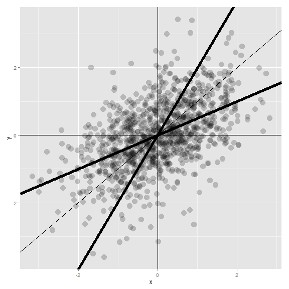
Let’s investigate the plot and the regression fits. If you had to predict a son’s normalized height, it would be \(Cor(Y, X) * X_i\) where \(X_i\) was the normalized father’s height. Conversely, if you had to predict a father’s normalized height, it would be \(Cor(Y, X) * Y_i\).

Multiplication by this correlation shrinks toward 0 (regression toward the mean). It is in this way that Galton used regression to account for regression toward the mean. If the correlation is 1 there is no regression to the mean, (if father’s height perfectly determines child’s height and vice versa).

Note since Galton’s original seminal paper, the idea of regression to the mean has been generalized and expanded upon. However, the core remains. In paired measurements, if there’s randomness then the extreme values of one element of the pair will be likely less extreme in the other element.

The number of applications of this phenomena is staggering. Some financial advisors recommend putting your money in your worst performing fund because of regression to the mean. (If there’s a lot of noise, those are the most likely to gain in value.) An example that I’ve run into is that students performing the best on midterm exams often do much worse on the final. Athletes often follow a phenomenal season with merely a good season. It’s a useful exercise to think whenever paired observations are being evaluated whether real intrinsic properties are being discussed, or just regression to the mean.

Exercises

1. You have two noisy scales and a bunch of people that you’d like to weigh. You weigh each person on both scales. The correlation was 0.75. If you normalized each set of weights, what would you have to multiply the weight on one scale to get a good estimate of the weight on the other scale? Watch a video solution.
2. Consider the previous problem. Someone’s weight was 2 standard deviations above the mean of the group on the first scale. How many standard deviations above the mean would you estimate them to be on the second? Watch a video solution.
3. You ask a collection of husbands and wives to guess how many jellybeans are in a jar. The correlation is 0.2. The standard deviation for the husbands is 10 beans while the standard deviation for wives is 8 beans. Assume that the data were centered so that 0 is the mean for each. The centered guess for a husband was 30 beans (above the mean). What would be your best estimate of the wife’s guess? Watch a video solution.