Symbolic Math: Differentiate and Integrate

Neural networks operate on numeric parameters adjusted by gradient descent. Symbolic mathematics, by contrast, operates by manipulating symbolic expressions.

This chapter implements a small symbolic mathematics core in Scala 3: terms, polynomials, exact differentiation, and exact integration. There are no numeric approximations, no step size to tune, and no truncation error. The rules of calculus are encoded directly, and every result is an exact expression.

All code is in source-code/symbolic-math.

Most calculus software used in machine learning is numeric. It represents a function as code and estimates its slope by perturbing the input by a small amount:

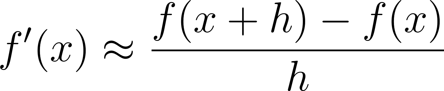
This finite difference is simple to implement and applies to any function that can be evaluated, which is why it is ubiquitous in numerical work. The limitation is the approximation itself. If 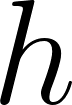is too large, curvature biases the estimate. If is too small, cancellation between two nearly equal numbers destroys precision. No single value of is suitable for every function, and the result is always a decimal rather than a formula.

Symbolic calculus takes the opposite approach. It represents an expression as data, a tree of operators and symbols, and rewrites that tree using the standard rules of calculus. Differentiating returns the exact expression 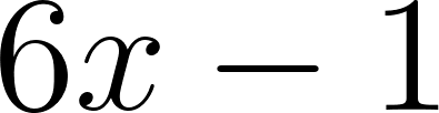, not a table of slopes. Evaluating that expression at a point is a separate, optional step. Because the manipulation is exact, symbolic methods expose structure that numeric methods conceal: the location of zeros of the derivative, the form of the antiderivative, and the relationship between two expressions.

Symbolic manipulation is one of the oldest branches of artificial intelligence. Systems such as Macsyma at MIT in the 1960s, and later Mathematica, Maple, and SymPy, were built to perform algebra symbolically, and much of that lineage was written in Lisp. The code in this chapter is a direct port of a small Common Lisp calculus package, and it follows the same principle: represent the mathematics as data, then apply rewrite rules.

For AI in particular, symbolic differentiation is the precursor to automatic differentiation, the technique underlying every deep learning framework. Automatic differentiation applies the same rules (power, sum, product, chain) mechanically to a program while carrying numeric values through the computation. Understanding the symbolic core makes the autodiff engine easier to reason about. The implementation here is deliberately small, and the chapter closes by noting what a full computer algebra system would add.

We start with the objects we can represent exactly. A term is a coefficient times a variable raised to a whole-number power:

A polynomial in one variable is a sum of such terms:

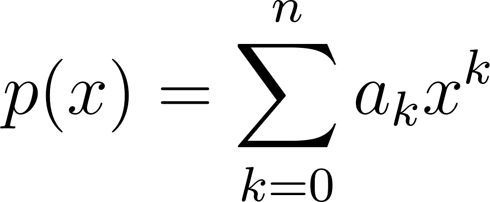
This representation covers a substantial part of introductory calculus and makes every rule exact. It consists of two case classes: one for a term and one for the polynomial that holds a list of terms. The complete data model, in Expr.scala, is as follows:

The design mirrors the algebra. Variable is a name, which allows the code to reject an attempt to add a polynomial in to one in rather than producing an invalid result. Term bundles the three values that define a monomial and provides negate and scale, the only two operations a term requires in this chapter. Polynomial holds the variable and a list of terms, and its companion object provides the three constants the algebra requires: zero, an arbitrary constant, and the identity .

The central method is normalize, and it must be understood before any calculus is attempted. When polynomials are added or scaled, the term list can contain like terms, terms with the same exponent, and terms whose coefficients cancel to zero. The raw list is correct but not canonical, so two polynomials that are mathematically equal may have different term lists. This breaks structural equality, and d/dx(int(p)) == p would fail even when the mathematics is correct.

normalize restores a canonical form in three steps:

1. groupBy(_.exponent) collects terms that share an exponent.
2. mapValues(_.map(_.coefficient).sum) adds their coefficients, so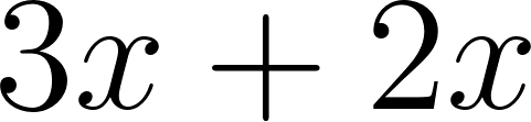 becomes .
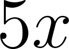3. The result is filtered to drop any coefficient equal to zero, then sorted by descending exponent.

After normalization, becomes the empty term list, which prints as 0, and prints as . Sorting by descending exponent places the highest power first, the conventional order for polynomials. This is what allows the test suite to compare whole polynomials with ==: equal polynomials have equal normalized term lists.

The remainder of the class is small and purely functional. degree reports the largest exponent, or zero for the zero polynomial. add verifies that both polynomials share a variable, concatenates the term lists, and normalizes. subtract negates the second polynomial and adds. scale multiplies every coefficient. evaluate computes the numeric value at a point using math.pow, which handles fractional and negative inputs correctly because the exponent is an integer. Every method returns a new value and leaves the receiver unchanged, so a sequence of rewrites is safe to reason about.

The toString implementations contain two notable details. First, a coefficient that is a whole number is printed without a decimal point, so 5.0 prints as 5 while 0.5 prints as 0.5. Second, a term of exponent 0 prints as the bare coefficient, exponent 1 prints as 6x, and higher powers print as 3x^2. The polynomial joins terms with " + " and then replaces "+ -" with "- ", so negative coefficients appear as subtraction. This substitution is why 6x - 1 appears instead of 6x + -1.

The derivative measures the instantaneous rate of change, defined by the limit

For a power of the variable, expanding 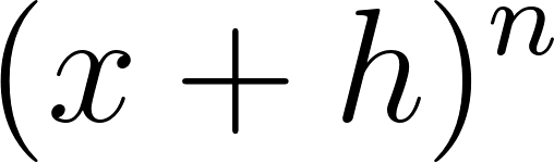with the binomial theorem and letting go to zero leaves exactly one surviving term, which gives the power rule:

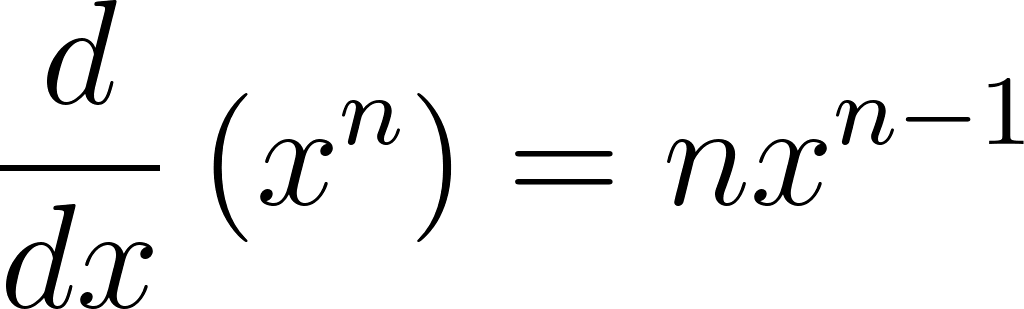
A constant multiple pulls out, and a sum differentiates term by term, the sum rule:

Together these two rules say differentiation is a linear operator, and they are all a polynomial needs. The code applies them per term, then collects the results. Here is Differentiate.scala in full:

differentiateTerm implements the power rule directly. It multiplies the coefficient by the exponent and decrements the exponent. A constant term has exponent zero, and its derivative is zero, so the function returns None rather than a term with a zero coefficient. That choice lets differentiate use flatMap, which transforms each term and discards the None results in a single pass. The Option return type expresses that a term either survives differentiation or vanishes.

differentiate applies that rule to every term and normalizes the survivors. The explicit if terms.isEmpty branch returns the zero polynomial when the input was constant; normalize would reach the same state, but the branch makes the intent clear. differentiateN applies the operator times by recursion, with a require guard that rejects a negative order. Its base case returns the polynomial unchanged, since the zeroth derivative of a function is the function itself.

The last two methods connect the symbolic representation to numeric values. gradientAt differentiates symbolically and then evaluates the exact derivative at a point, so the slope is computed from a formula rather than a finite difference. criticalPoint tests whether that slope is zero within a tolerance, the condition for a local maximum, minimum, or saddle point. For the derivative is , which is zero at 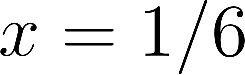, the vertex of the upward parabola. The test suite checks that point explicitly.

Integration runs the power rule backward. Since differentiating 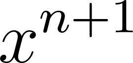multiplies by 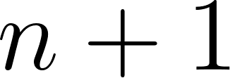, integrating must divide by it:

The added is the constant of integration. Any constant differentiates to zero, so an antiderivative is defined only up to an additive constant, and a complete answer must state it. The code returns the antiderivative with 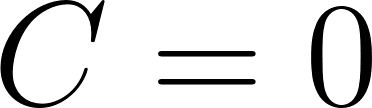and lets the caller add when printing. For polynomials with non-negative exponents, is at least one, so the division is always defined. Like differentiation, integration is linear and applies term by term.

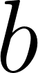
A definite integral goes from a lower limit to an upper limit . The fundamental theorem of calculus says the answer is the antiderivative evaluated at the endpoints:

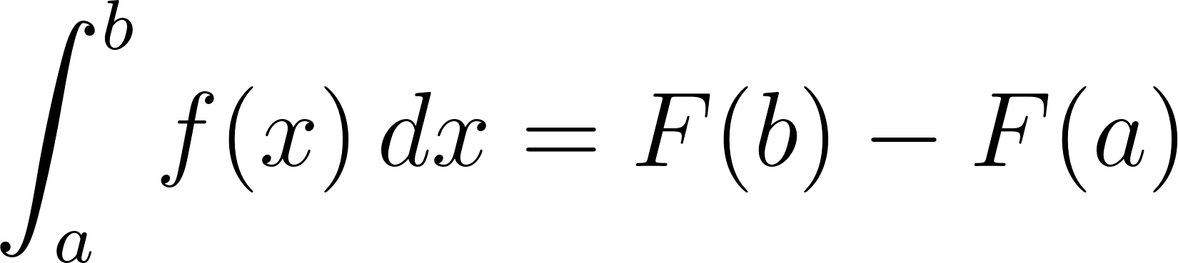
The constant of integration cancels in the subtraction, which is why the code never has to track it. Here is Integrate.scala in full:

integrateTerm increments the exponent and divides the coefficient by the new exponent. It always returns a Term, never an Option, because no polynomial term integrates to zero. integrate applies it across the terms and normalizes. integrateN repeats the operation for higher antiderivatives, with the same non-negative guard as differentiateN. definite integrates once to obtain an antiderivative, then subtracts its value at from its value at , following the theorem directly.

The two operators are inverse in one direction. Differentiating an antiderivative returns the original polynomial, so the test suite asserts Differentiate.differentiate(Integrate.integrate(p)) == p. The reverse order holds only up to the constant: integrating a derivative returns the original plus an unknown , so no such equality is asserted in the other direction. This asymmetry is precisely why the constant of integration exists.

Main.scala exercises every operation on a single polynomial:

The polynomial is constructed from an explicit list of terms and normalized, so the printed order is canonical. The demo prints the polynomial, its first and second derivatives, its indefinite integral (with the + C appended by the print statement rather than the library), a definite integral, and a point evaluation. Running it from the example directory:

produces:

The project includes a self-checking test file that requires no test framework. It uses plain assert calls and a small close helper for floating point comparisons:

The checks target the important behavior rather than coverage. The first two confirm the power rule and the sum rule on a concrete polynomial. The zeroth-derivative check confirms the base case of the recursion. The constant check confirms that a term of exponent zero disappears entirely, leaving an empty term list. The integration checks confirm the reverse power rule symbolically and the fundamental theorem numerically. The round trip is the strongest test in the file: it exercises both operators across all three terms and would catch an error in either rule. The final numeric checks connect the symbolic derivative back to the geometry, confirming 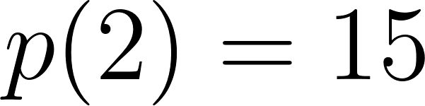, 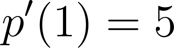, and that is a critical point.

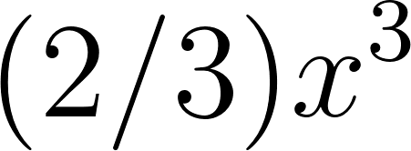
The close helper compares doubles within a tolerance rather than for exact equality. This is the correct approach for floating point arithmetic: 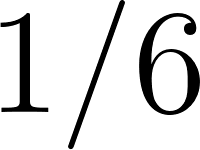is not exactly representable, and an antiderivative such as produces a repeating decimal. Exact comparison would fail on rounding error unrelated to the logic. The tolerance is 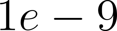for these small numbers, loose enough to absorb representation error and tight enough to detect a genuine mistake.

Run it with:

and it prints one line:

The demo output demonstrates that the rules agree with hand calculus.

p = 3x^2 - 1x + 5 is the input polynomial. The 1x is the coefficient-one term printed literally, a minor cosmetic limitation of toString. The mathematics is correct; a more careful printer would omit the 1 and write x, which is left as an exercise.

p' = 6x - 1 applies the power rule to each term: 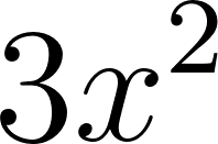gives 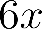, 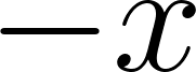gives 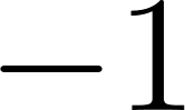, and the constant 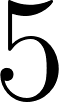gives nothing. The sum of those results is the exact derivative, with no decimal approximation.

p'' = 6 differentiates once more. The term becomes 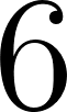and the term disappears. The second derivative of a quadratic is constant, the algebraic statement that its slope changes at a constant rate.

int(p) = 1x^3 - 0.5x^2 + 5x + C reverses the process term by term: integrates to 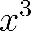, to 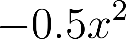, and to . The 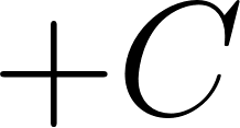is appended by the demo because the library returns the antiderivative. Omitting is common in software but a frequent source of error, so the print statement makes it explicit.

int[0,2] = 16.0 evaluates the antiderivative at the endpoints. Substituting 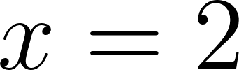gives and substituting 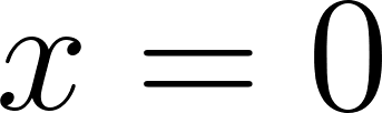gives , so the definite integral is 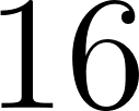. This is the signed area under the curve between the two limits. The test file checks the simpler case 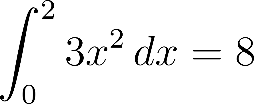with the same machinery.

p(2) = 15.0 is a direct evaluation: . This value does not involve calculus and confirms that evaluate agrees with arithmetic.

Taken together, the output shows the three requirements of a computer algebra system: rewrite an expression exactly, evaluate the result at a point, and remain consistent across inverse operations. The round-trip test verifies the last property.

The limits of a small system are as important as its features, because they define the starting point for any larger implementation.

• One variable only. Every polynomial carries a single Variable, and add refuses to mix variables. Multivariate polynomials would need a term to hold a monomial over several variables, and differentiation would become a partial derivative that names the variable to differentiate.
• Polynomials only. There is no product rule, quotient rule, or chain rule, because there are no products, quotients, or compositions in the data model. Adding those rules means replacing the flat term list with a general expression tree whose nodes are Add, Mul, Pow, Sin, and so on. The pattern matching style carries over unchanged.
• No simplification beyond collecting like terms. normalize combines coefficients, but it does not expand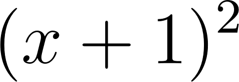 , factor 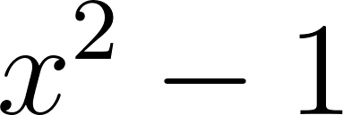, or cancel rational expressions. Each of those is a separate rewrite system.
• The exponent is not constrained. Nothing stops a caller from constructing . Differentiation handles it, but integration divides by and would divide by zero. A require in the Term constructor or a check in integrateTerm would close the gap.
• Floating point coefficients. Coefficients are Double, so a coefficient like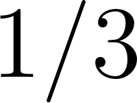 is inexact. Collecting like terms compares against 0.0 with exact equality, which is safe for the halves and thirds produced by these rules but could misjudge a true cancellation that arrives by two rounding paths. A rational number type would make the algebra exact.

Each of these is a deliberate trade. The value of the small core is that every limitation is visible within a few dozen lines, and each has a clear path to a more capable implementation.

This chapter implemented a working computer algebra core in pure Scala with no dependencies. The components are small, but together they cover the full path from representation to verification.

• Terms and polynomials as case classes turn algebra into data. normalize restores a canonical form, which is what makes exact structural equality, and therefore round-trip testing, possible.
• Differentiation is the power rule plus linearity. differentiateTerm returns an Option so vanishing constants are removed by flatMap, and differentiateN composes the rule for higher orders.
• Integration is the reverse power rule plus the fundamental theorem of calculus. The constant of integration is dropped because the definite integral cancels it, and the round trip differentiate(integrate(p)) == p verifies that the two rules are inverse.
• The test suite verifies each rule with a concrete value and one cross-check, using a tolerance for the floating point comparisons that exact equality cannot survive.

The broader point concerns representation. Here calculus is not a collection of formulas to memorize but a set of rewrite rules acting on a type. The same structure, small immutable value types with companion-object operations and pure functions, reappears later in this book for search states, grammar tags, and graph triples. When a later chapter addresses automatic differentiation or a neural-symbolic system, the symbolic component is the machinery built here, scaled up.

1. Nicer printing. The demo prints 1x^3 and 1x where a mathematician writes x^3 and x. Modify Term.toString so a coefficient of 1 is omitted (except for a constant term, where it must still print), and update the assertion in symbolicMathTest that expects 1x^3.

2. Guard the exponent. Add require(exponent >= 0, "Exponent must be non-negative.") to the Term case class. Confirm the existing tests still pass, then try constructing Term(1.0, Variable("x"), -1) and report the error. Explain why the guard is better placed on the type than inside Integrate.integrateTerm.

3. Multiply two polynomials. Add def multiply(other: Polynomial): Polynomial to Polynomial. Multiply term by term, add the exponents and multiply the coefficients, and normalize the result. Test it on and confirm the answer is . Why can you not express this with the existing add and scale alone?

4. Check the derivative against a finite difference. Write a function finiteDifference(p: Polynomial, x: Double, h: Double): Double that computes , and compare it to for at 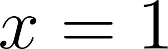with , 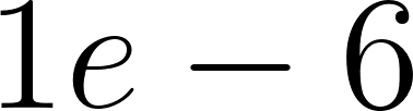, and 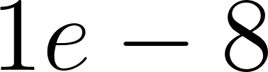. Report the error at each step and explain why it eventually gets worse as shrinks.

5. Numeric integration for comparison. Implement a Riemann sum or Simpson’s rule that approximates 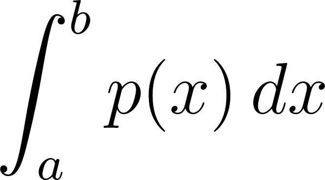from evaluations of . Compare it to Integrate.definite for on 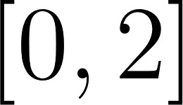and report the difference. Which method would you trust for a polynomial and why?

6. Second derivative test. Add a function classifyCriticalPoint(p: Polynomial, x: Double): String that returns "minimum", "maximum", or "inflection" using the sign of the second derivative. Test it at for and confirm it reports a minimum.

7. Higher-order round trip. Assert that for 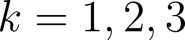on a polynomial of degree at least three. Does the identity hold for every 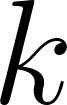? Explain the role of the dropped constants.

8. A general expression tree. Replace the flat polynomial with a sealed trait Expr and cases Const, Var, Add, Mul, and Pow. Implement derivative using the sum, product, and power rules. Test it on and compare the result to differentiating directly. What extra simplification would you need to make the two answers print identically?