Probability: Bayes, Base Rates, and Tests
Probability is the language AI uses to reason under uncertainty. A spam filter asks how likely a message is junk given the words it contains. A medical system asks how likely a patient is sick given a test result. A model evaluation asks whether an observed improvement is real or just noise. Each of those is a probability question wearing different clothes.
Many developers use probability through a library and never derive it, which works until a result looks wrong and there is no intuition to check it against. This chapter builds the machinery from scratch in pure Scala 3 so the formulas stay visible. It covers the two main schools of thought. Bayesian reasoning treats probability as a degree of belief and revises that belief when evidence arrives. Frequentist reasoning treats probability as a long-run frequency and asks how surprising the data would be if a null claim were true. It closes with correlation, the most used and most abused single number in data work.
All code is in source-code/probability. The project has no dependencies beyond the Scala standard library, so every formula is ours to read.
Two Ways to Read a Probability
Before the formulas, fix the vocabulary. A sample space 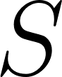 is the set of all possible outcomes, such as the two sides of a coin or the six faces of a die. An event
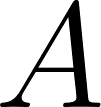 is a subset of . A probability
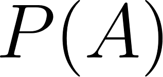 assigns a number in
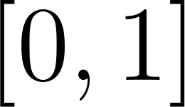 to each event, with
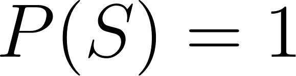 and, for disjoint events,
 . A random variable is a function from outcomes to numbers, so “number of heads in ten tosses” is a random variable even though the outcomes are sequences of coin faces.
The first useful idea is conditional probability, the chance of given that 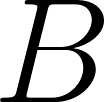 happened:
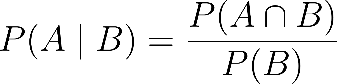
We divide by 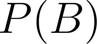 because once we know occurred, the only outcomes left are those inside , and becomes our new universe. Rearranging gives the product rule
 , and applying it both ways gives the equation that powers this whole chapter.
The same numbers carry two different meanings. A frequentist reads  as a statement about a long run of tosses: about half come up heads. A Bayesian reads it as a degree of belief, something that can be updated as evidence arrives. The arithmetic is identical. Only the interpretation and the willingness to state a prior differ, and that difference drives the split between the next two sections.
Bayes Theorem
Conditional probability is symmetric in a specific way. The chance of given and the chance of given are linked by the product rule:

Solving for 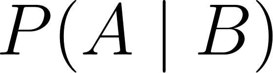 gives Bayes theorem:
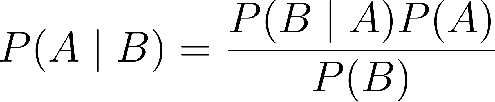
Read as a hypothesis 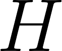 and as evidence
 and the four named parts appear:
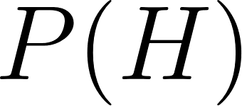 is the prior, what we believed before seeing the evidence.
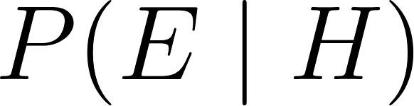 is the likelihood, how well the hypothesis predicts the evidence.
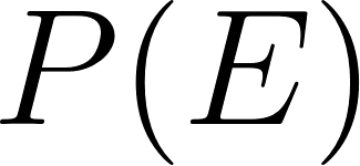 is the marginal likelihood (or evidence), the total chance of seeing under every hypothesis.
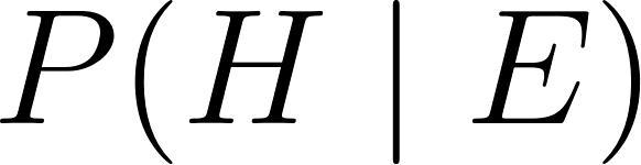 is the posterior, what we believe after the evidence.
When there are several competing hypotheses, the marginal is the sum over all of them, which is exactly how the code normalizes:

That sum is the key. It is what forces the posteriors to add up to one, and it is why a strong test can still produce a weak posterior when the alternatives are numerous or likely. The denominator is where base rates do their work.
Bayes in Seven Lines
The implementation splits cleanly into a value type and a companion object. The value type holds a normalized map from hypothesis name to probability. The object holds the two operations, constructing a model from priors and updating it with evidence. Here is the complete file:
 1 //> using scala 3.6.4
 2 // Copyright 2026 Mark Watson. All rights reserved.
 3
 4 package probability
 5
 6 // Bayes model: a normalized map of hypothesis -> probability.
 7 // Port of bayes.lisp: P(H|E) = P(E|H) * P(H) / sum_h P(E|h) * P(h)
 8 final case class BayesModel(posteriors: Map[String, Double]):
 9   def posterior(hypothesis: String): Double =
10     posteriors.getOrElse(
11       hypothesis,
12       throw new NoSuchElementException(s"Hypothesis $hypothesis not found in model.")
13     )
14   def map: (String, Double) = posteriors.maxBy(_._2)
15
16 object BayesModel:
17   def fromPriors(priors: Map[String, Double]): BayesModel =
18     val total = priors.values.sum
19     require(total > 0.0, "All priors are zero, cannot normalize.")
20     BayesModel(priors.view.mapValues(_ / total).toMap)
21
22   def update(
23       model: BayesModel,
24       evidence: String,
25       likelihood: (String, String) => Double
26   ): BayesModel =
27     val unnorm = model.posteriors.map { case (h, prior) => h -> likelihood(h, evidence) * prior }
28     val marginal = unnorm.values.sum
29     require(marginal > 0.0, "Marginal likelihood is zero, evidence is impossible under all hypotheses.")
30     BayesModel(unnorm.view.mapValues(_ / marginal).toMap)
Walk through it line by line.
fromPriors divides every prior by their sum. This means the caller can pass raw counts, rates, or anything proportional and still get a valid distribution. A prior map of Map("disease" -> 1, "healthy" -> 999) normalizes to the same model as Map("disease" -> 0.001, "healthy" -> 0.999). Accepting unnormalized input is a small kindness that removes a whole class of caller mistakes.
update is the heart of the file. It maps over the current posteriors, multiplies each prior by likelihood(h, evidence), and collects the results in unnorm. Those numbers are proportional to the true posteriors but do not sum to one, so the next line sums them into marginal and divides. The map is rebuilt with BayesModel(...) so a new immutable value is returned and the old model is untouched. Updating twice is just calling update twice, which is exactly what a Bayesian agent does when evidence arrives in sequence.
The require calls mark the two ways Bayes can fail. If every prior is zero, the prior map was empty or nonsense and there is nothing to normalize. If the marginal is zero, the evidence is impossible under every hypothesis, so no amount of updating can explain it. Both are caller errors rather than data problems, so the code fails loudly with a clear message instead of returning a map of NaN values that would silently poison everything downstream.
The posterior method reads one hypothesis by name and throws a named exception if it is missing, which turns a typo into an immediate error. The map method returns the maximum a posteriori hypothesis, the single most likely one, which is the natural output when a system must commit to a decision. Note that the most likely hypothesis is not the same as a confident one. As the medical example shows, the MAP can be “healthy” while the probability of disease is still far from zero.
The Medical Test That Fools Doctors
This is the most famous counterintuitive result in applied probability, and the code demo exists to make it concrete. A rare disease affects 0.1% of a population. A screening test detects 99% of true cases (its sensitivity), but it also returns a false positive 5% of the time. A patient tests positive. What is the chance she actually has the disease?
Almost everyone, including many physicians asked in real studies, answers “about 99%.” The correct answer is about 1.9%. The reason is that the healthy group is enormous, so even a small false-positive rate produces far more false positives than the tiny sick group produces true positives.
Do the arithmetic by hand first. Take a population of 100,000 people.
| Group | Count | Test positive | True positives | False positives |
|---|---|---|---|---|
| Disease | 100 | 99% | 99 | |
| Healthy | 99,900 | 5% | 4,995 |
Out of 100,000 people, about 99 + 4,995 = 5,094 test positive, and only 99 of those actually have the disease. The share is  , or 1.94%. The false positives outnumber the true positives roughly fifty to one. This is the base rate fallacy: people anchor on the test’s accuracy and ignore how rare the condition is.
The same numbers fall straight out of Bayes. The unnormalized products are  for disease and
 for healthy. Their sum, the marginal, is
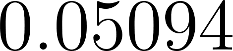 . Dividing gives
 for disease and
 for healthy. The likelihood ratio of 99 to 5, about 20 to 1, is strong, but the prior ratio of 1 to 999 is far stronger in the other direction, and the prior wins.
Here is the demo that runs these numbers, in full:
 1 //> using scala 3.6.4
 2 // Copyright 2026 Mark Watson. All rights reserved.
 3
 4 package probability
 5
 6 // Medical screening case from Probability/examples/medical.lisp.
 7 // A rare disease hits 0.1% of people. The test catches 99% of cases
 8 // but gives false positives 5% of the time. Given a positive test,
 9 // the chance of disease is only about 1.9%.
10 @main def probabilityDemo(): Unit =
11   val prevalence = 0.001
12   val sensitivity = 0.99
13   val falsePositiveRate = 0.05
14
15   def likelihood(hypothesis: String, evidence: String): Double =
16     hypothesis match
17       case "disease" => sensitivity
18       case "healthy" => falsePositiveRate
19       case h => throw new IllegalArgumentException(s"Unknown hypothesis: $h")
20
21   val prior = BayesModel.fromPriors(Map("disease" -> prevalence, "healthy" -> (1.0 - prevalence)))
22   val updated = BayesModel.update(prior, "positive-test", likelihood)
23
24   println("=== Bayesian Analysis: Medical Screening Test ===")
25   println("Priors:")
26   prior.posteriors.foreach { case (h, p) => println(f"  P($h) = $p%.4f") }
27   println("After a POSITIVE test result:")
28   updated.posteriors.foreach { case (h, p) => println(f"  P($h | positive) = $p%.4f (${p * 100}%.2f %%)") }
29   println(s"MAP hypothesis: ${updated.map._1}")
30   println("Despite 99% sensitivity, a positive test gives only about 1.9%")
31   println("chance of disease because the disease is so rare.")
32
33   val (z, pValue) = Frequentist.zTestProportion(60, 100, 0.5)
34   println(f"\nCoin toss check: 60 heads in 100 tosses vs fair coin: z = $z%.3f, p = $pValue%.4f")
35   val (lo, hi) = Frequentist.wilsonInterval(60, 100)
36   println(f"95%% Wilson interval for the bias: [$lo%.3f, $hi%.3f]")
The likelihood function is the one piece the caller supplies. It ignores the evidence string here because there is only one kind of evidence in this demo, a positive test, but the signature (String, String) => Double is general enough to score any evidence against any hypothesis. The pattern match ends with a wildcard case that throws, so a misspelled hypothesis name is caught at the moment of use rather than silently treated as zero. The f string interpolator with %.4f keeps the printed columns aligned, and %% prints a literal percent sign.
One update is a good start, but the interesting behavior appears with a second test. A second positive result is treated as independent evidence, so we call update again on the already updated model. The prior for the second update is the posterior from the first, which is the entire point of Bayesian updating: yesterday’s belief becomes today’s starting point. After two positive tests the chance of disease rises from about 1.9% to about 28%. That is still not a diagnosis, but it changes the decision completely, which is why a good doctor orders a confirmatory test instead of celebrating or panicking after one result. The test file checks exactly this monotonic rise.
Frequentist Checks: z, Chi-Squared, Wilson
Bayes gives a clean answer but demands a prior, and sometimes no honest prior exists. The frequentist toolkit takes a different route. It does not assign probabilities to hypotheses at all. Instead it states a null hypothesis, a default claim such as “the coin is fair,” and asks how likely the observed data would be if that claim were true. If the data would be very unlikely, we reject the null. The output of a test is a p-value, the chance of seeing data at least this extreme under the null.
The subtle point, repeated in the code comments because it is so often gotten wrong, is what a p-value is not. A small p-value says the data would be rare if the null were true. It does not say the null has a small probability of being true. Those are different statements, and swapping them is the most common error in applied statistics. With that warning in place, here is the complete file:
 1 //> using scala 3.6.4
 2 // Copyright 2026 Mark Watson. All rights reserved.
 3
 4 package probability
 5
 6 // Frequentist toolkit: z-tests, chi-squared tests, confidence intervals.
 7 // Port of frequentist.lisp. A small p-value says the data would be
 8 // unlikely if the null were true. It does not give P(null is false).
 9 object Frequentist:
10
11   // Standard normal CDF via Abramowitz and Stegun 26.2.17, error < 1.5e-7.
12   def phiApprox(z: Double): Double =
13     val p = 0.2316419
14     val b1 = 0.319381530
15     val b2 = -0.356563782
16     val b3 = 1.781477937
17     val b4 = -1.821255978
18     val b5 = 1.330274429
19     val az = math.abs(z)
20     val t = 1.0 / (1.0 + p * az)
21     val pdf = math.exp(-0.5 * az * az) / math.sqrt(2.0 * math.Pi)
22     val cdf = 1.0 - pdf * (b1 * t + b2 * t * t + b3 * t * t * t + b4 * t * t * t * t + b5 * t * t * t * t * t)
23     if z >= 0.0 then cdf else 1.0 - cdf
24
25   // Chi-squared CDF via the Wilson-Hilferty transform, then phiApprox.
26   def chiSquaredCdf(x: Double, df: Int): Double =
27     if x <= 0.0 then 0.0
28     else
29       val k = df.toDouble
30       val term = 2.0 / (9.0 * k)
31       val z = (math.pow(x / k, 1.0 / 3.0) - (1.0 - term)) / math.sqrt(term)
32       phiApprox(z)
33
34   def zScore(observed: Double, expected: Double, stdDev: Double): Double =
35     require(stdDev > 0.0, "stdDev must be positive.")
36     (observed - expected) / stdDev
37
38   // One-sample z-test for a binomial proportion. Returns (z, two-tailed p).
39   def zTestProportion(successes: Int, n: Int, hypothesisedP: Double): (Double, Double) =
40     val pHat = successes.toDouble / n
41     val se = math.sqrt(hypothesisedP * (1.0 - hypothesisedP) / n)
42     val z = (pHat - hypothesisedP) / se
43     (z, math.min(2.0 * (1.0 - phiApprox(math.abs(z))), 1.0))
44
45   // Pearson chi-squared goodness of fit. Returns (chi2, df, p).
46   def chiSquaredTest(observed: Seq[Double], expected: Seq[Double]): (Double, Int, Double) =
47     require(observed.size == expected.size, "Observed and expected must have the same length.")
48     val chi2 = observed.zip(expected).map { case (o, e) =>
49       if e == 0.0 then 0.0 else (o - e) * (o - e) / e
50     }.sum
51     val df = observed.size - 1
52     (chi2, df, math.max(1.0 - chiSquaredCdf(chi2, df), 0.0))
53
54   // Inverse normal CDF via Acklam's approximation, error < 1.2e-9.
55   def inversePhi(p: Double): Double =
56     require(p > 0.0 && p < 1.0, "p must lie strictly between 0 and 1.")
57     val a = Array(-3.969683028665376e+01, 2.209460984245205e+02, -2.759285104469687e+02, 1.383577518672690e+02, -3.066479806614716e+01, 2.506628277459239e+00)
58     val b = Array(-5.447609879822406e+01, 1.615858368580409e+02, -1.556989798598866e+02, 6.680131188771972e+01, -1.328068155288572e+01)
59     val c = Array(-7.784894002430293e-03, -3.223964580411365e-01, -2.400758277161838e+00, -2.549732539343734e+00, 4.374664141464968e+00, 2.938163982698783e+00)
60     val d = Array(7.784695709041462e-03, 3.224671290700398e-01, 2.445134137142996e+00, 3.754408661907416e+00)
61     def poly(coef: Array[Double], x: Double): Double =
62       coef.foldLeft(0.0)((acc, c) => acc * x + c)
63     if p < 0.02425 then
64       val q = math.sqrt(-2.0 * math.log(p))
65       (((((c(0) * q + c(1)) * q + c(2)) * q + c(3)) * q + c(4)) * q + c(5)) /
66         ((((d(0) * q + d(1)) * q + d(2)) * q + d(3)) * q + 1.0)
67     else if p <= 0.97575 then
68       val q = p - 0.5
69       val r = q * q
70       (((((a(0) * r + a(1)) * r + a(2)) * r + a(3)) * r + a(4)) * r + a(5)) * q /
71         (((((b(0) * r + b(1)) * r + b(2)) * r + b(3)) * r + b(4)) * r + 1.0)
72     else
73       val q = math.sqrt(-2.0 * math.log(1.0 - p))
74       -(((((c(0) * q + c(1)) * q + c(2)) * q + c(3)) * q + c(4)) * q + c(5)) /
75         ((((d(0) * q + d(1)) * q + d(2)) * q + d(3)) * q + 1.0)
76
77   // Wilson score interval for a binomial proportion. Returns (lo, hi).
78   def wilsonInterval(successes: Int, n: Int, confidence: Double = 0.95): (Double, Double) =
79     val z = inversePhi((1.0 + confidence) / 2.0)
80     val pHat = successes.toDouble / n
81     val denom = 1.0 + z * z / n
82     val center = (pHat + z * z / (2.0 * n)) / denom
83     val half = z * math.sqrt(pHat * (1.0 - pHat) / n + z * z / (4.0 * n * n)) / denom
84     (math.max(center - half, 0.0), math.min(center + half, 1.0))
Everything here rests on the standard normal distribution, the bell curve with mean 0 and variance 1. Its cumulative distribution function, written 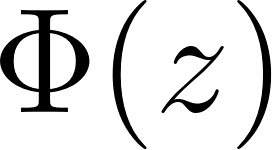 , gives the probability that a normal random variable is at most
 . There is no closed form for
 , so the code uses a rational approximation from Abramowitz and Stegun (formula 26.2.17) that is accurate to about
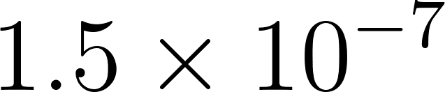 . The approximation is written for the upper tail of the positive side, so
phiApprox computes the value for 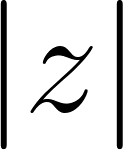 and then mirrors it with
1 - cdf for negative to respect the symmetry of the bell curve. The five constants 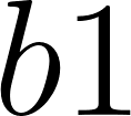 through
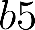 are the coefficients of the fitted polynomial in
 , a change of variable that keeps the fit well behaved far out in the tails.
chiSquaredCdf reuses phiApprox through the Wilson-Hilferty transform, which says a chi-squared variable with 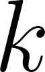 degrees of freedom behaves roughly like a cube root of a normal. The transform maps the chi-squared value
 to a z-score, then feeds it to
phiApprox. This is why one small normal routine supports two very different tests.
zTestProportion is the coin-toss check. For a proportion, the standard error under the null is  , and the z-score measures how many standard errors the observed rate sits from the hypothesized rate:
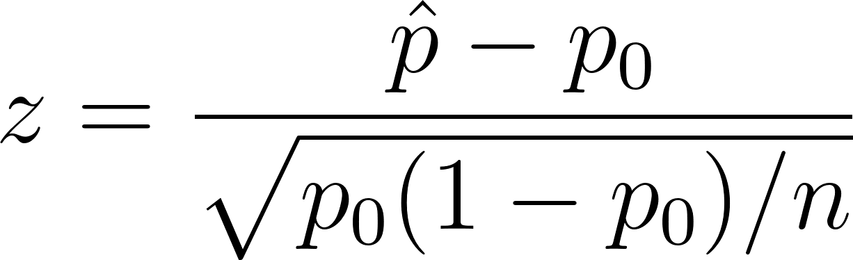
The p-value is two-tailed,  , because a coin that is biased in either direction is equally interesting, and it is capped at 1.0 so rounding can never produce a probability above one.
chiSquaredTest handles more than two categories. It compares each observed count to its expected count, sums the squared relative gaps, and sets the degrees of freedom to one less than the number of categories:
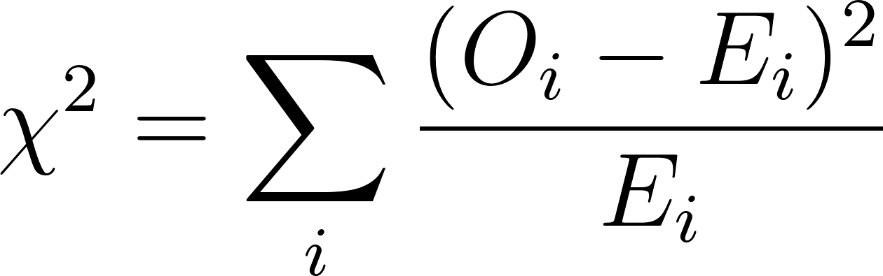
The guard if e == 0.0 then 0.0 avoids dividing by zero. The final p-value is the upper tail  , clamped at zero for the same reason the z-test p-value is clamped at one.
inversePhi goes the other way, from a probability to a z-score, using Acklam’s approximation with three polynomial regions and a Horner-style poly fold. We need it for confidence intervals, where the multiplier is the z-score that leaves a given tail area. For 95% confidence the code calls inversePhi(0.975) and gets 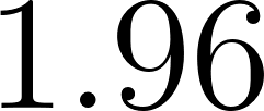 , the number every statistics course makes you memorize.
The Wilson interval is the payoff. A naive confidence interval for a proportion uses the same standard error as the z-test,  . That is the Wald interval, and it fails badly near 0 and 1, sometimes producing bounds outside or a zero-width interval when you observe no successes. The Wilson interval solves the quadratic that the Wald interval linearizes, which pulls the center toward 0.5 and adds
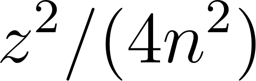 inside the square root. The result is always inside , and the code enforces that with
math.max and math.min. For 60 heads in 100 tosses the Wilson interval is about  , a range you can read with no test lore: the data are consistent with a fair coin, but also with a genuine bias up to about 69%.
Correlation in Nine Lines
The last tool is the one most likely to mislead. Correlation measures how strongly two series move together. It begins with covariance, the average product of each pair’s deviations from their own means:

If and  tend to be above their means at the same time, the products are mostly positive and the covariance is positive. If one is high while the other is low, it is negative. The problem is that covariance carries the units of the data, so a covariance of 500 means nothing on its own. Dividing by both spreads fixes that and produces the Pearson correlation coefficient:
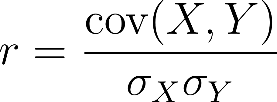
Here is the complete file:
 1 //> using scala 3.6.4
 2 // Copyright 2026 Mark Watson. All rights reserved.
 3
 4 package probability
 5
 6 // Correlation helpers. Port of correlation.lisp.
 7 object Correlation:
 8   def mean(xs: Seq[Double]): Double =
 9     require(xs.nonEmpty, "Cannot take the mean of an empty series.")
10     xs.sum / xs.size
11
12   def covariance(xs: Seq[Double], ys: Seq[Double]): Double =
13     require(xs.size == ys.size && xs.nonEmpty, "Series must be non-empty and equal in length.")
14     val mx = mean(xs)
15     val my = mean(ys)
16     xs.zip(ys).map { case (x, y) => (x - mx) * (y - my) }.sum / xs.size
17
18   def stdDev(xs: Seq[Double]): Double =
19     math.sqrt(covariance(xs, xs))
20
21   // Pearson r in [-1, 1]. Returns 0 when either series is constant.
22   def pearson(xs: Seq[Double], ys: Seq[Double]): Double =
23     val sx = stdDev(xs)
24     val sy = stdDev(ys)
25     if sx == 0.0 || sy == 0.0 then 0.0
26     else covariance(xs, ys) / (sx * sy)
The design is a small chain of reuse. mean guards against an empty series. covariance checks that the two series are the same non-empty length, computes both means, then zips the pairs and averages the products of deviations. stdDev calls covariance with the same series twice, because the covariance of a variable with itself is its variance, and takes the square root. pearson divides the covariance by the product of the two standard deviations.
Note that the variance here divides by  rather than
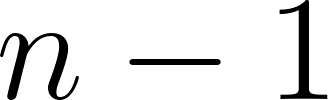 . That is the maximum likelihood form. For correlation it makes no difference at all, because the same appears in the numerator and both denominators and cancels. The choice only matters when you report a variance or standard deviation as a standalone estimate.
The pearson guard is the interesting line. If either series is constant, its standard deviation is zero and the division would produce 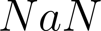 , a value that spreads silently through any computation that touches it. Rather than propagate a poison value, the function returns 0.0. That is a defensible convention, because a flat line carries no trend to track, so it has no linear relationship with anything. The test file pins both cases: a perfect line gives
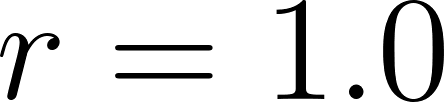 and a constant series gives 0.0.
The interpretation is where caution is required.  near 1 means the two series move together almost linearly, near -1 means they move in opposite directions, and near 0 means no linear relationship. It never means that one series causes the other. The medical example in this chapter is the proof. Test results and disease status are strongly correlated, yet a single positive test still implies only a small chance of disease, because the base rate is tiny. Correlation measures co-movement, not importance and not causation. A second trap is that captures only straight-line relationships: a perfect parabola can have
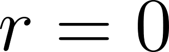 while is completely determined by . Always plot the data before trusting the number.
The Test Suite
The project includes a self-checking test file that runs without any test framework, using plain assert calls and a small close helper for floating point comparisons. Reading it is the fastest way to see the expected behavior of every function:
 1 //> using scala 3.6.4
 2 // Copyright 2026 Mark Watson. All rights reserved.
 3
 4 package probability
 5
 6 // Offline checks for the probability toolkit. Run with: scala-cli run . --main-class probability.probabilityTest
 7 @main def probabilityTest(): Unit =
 8   def close(a: Double, b: Double, tol: Double, label: String): Unit =
 9     assert(math.abs(a - b) <= tol, s"$label: expected $b, got $a")
10
11   // Bayes: priors normalize, medical posterior is about 1.94%.
12   val prior = BayesModel.fromPriors(Map("disease" -> 0.001, "healthy" -> 0.999))
13   close(prior.posteriors.values.sum, 1.0, 1e-12, "priors sum to 1")
14   val updated = BayesModel.update(prior, "positive-test",
15     (h, _) => if h == "disease" then 0.99 else 0.05)
16   close(updated.posterior("disease"), 0.01943, 1e-4, "medical posterior")
17   assert(updated.map._1 == "healthy", "MAP stays healthy after one positive test")
18   // Second positive test raises the chance a lot.
19   val twice = BayesModel.update(updated, "positive-test",
20     (h, _) => if h == "disease" then 0.99 else 0.05)
21   assert(twice.posterior("disease") > updated.posterior("disease"), "second positive raises posterior")
22
23   // Normal CDF spot checks.
24   close(Frequentist.phiApprox(0.0), 0.5, 1e-9, "phi(0)")
25   close(Frequentist.phiApprox(1.96), 0.975, 1e-3, "phi(1.96)")
26   close(Frequentist.inversePhi(0.975), 1.96, 1e-3, "inversePhi(0.975)")
27
28   // z-test on an obvious bias: 700 heads in 1000 tosses vs fair coin.
29   val (z, p) = Frequentist.zTestProportion(700, 1000, 0.5)
30   assert(z > 10.0 && p < 1e-9, s"biased coin must reject fair null, got z=$z p=$p")
31
32   // Chi-squared on near-uniform dice rolls: high p-value keeps the null.
33   val (_, _, pDice) = Frequentist.chiSquaredTest(
34     Seq(16.0, 18.0, 15.0, 17.0, 16.0, 18.0), Seq(16.67, 16.67, 16.67, 16.67, 16.67, 16.67))
35   assert(pDice > 0.5, s"fair dice must keep the null, got p=$pDice")
36
37   // Wilson interval covers the observed rate and stays in [0, 1].
38   val (lo, hi) = Frequentist.wilsonInterval(60, 100)
39   assert(lo <= 0.6 && 0.6 <= hi && lo >= 0.0 && hi <= 1.0, s"bad Wilson interval [$lo, $hi]")
40
41   // Correlation: perfect line gives r = 1, flat series gives 0.
42   close(Correlation.pearson(Seq(1.0, 2.0, 3.0, 4.0), Seq(2.0, 4.0, 6.0, 8.0)), 1.0, 1e-12, "pearson line")
43   close(Correlation.pearson(Seq(1.0, 1.0, 1.0), Seq(2.0, 4.0, 6.0)), 0.0, 1e-12, "pearson constant")
44
45   println("All probability tests passed.")
The close helper compares two doubles within a tolerance, which is the correct way to test floating point math. Comparing exact equality would fail on the rounding error that is unavoidable in a polynomial approximation. The tolerance is chosen per check: 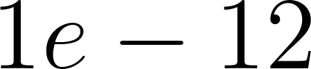 where the arithmetic is exact,
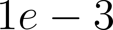 where an approximation is involved.
The checks are chosen to pin down the interesting behavior rather than to chase coverage. The prior check confirms normalization. The medical posterior check pins the 1.94% result. The MAP assertion confirms that a single positive test does not flip the decision. The second-update assertion confirms that evidence accumulates. The normal checks pin 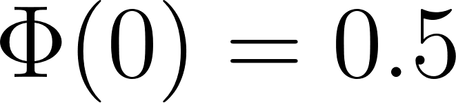 ,
 , and the inverse round trip. The biased coin case uses 700 heads in 1000 tosses, which is so far from fair that the z-score exceeds 10 and the p-value underflows past
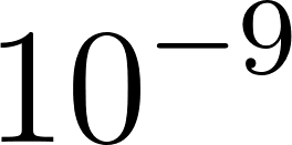 , an unambiguous rejection. The dice case is the opposite: near-uniform counts produce a high p-value, so the fair null is kept. The Wilson check confirms the interval brackets the observed rate and stays inside the legal range. The two correlation checks pin the perfect line and the constant-series guard.
Running the Examples
The project is driven by scala-cli, which compiles and runs a directory of Scala sources with no build file. Run the interactive demo and the test suite from the example directory:
1 cd source-code/probability
2 scala-cli run . --main-class probability.probabilityDemo
3 scala-cli run . --main-class probability.probabilityTest
The demo prints the Bayesian screen followed by the two frequentist checks:
 1 === Bayesian Analysis: Medical Screening Test ===
 2 Priors:
 3   P(disease) = 0.0010
 4   P(healthy) = 0.9990
 5 After a POSITIVE test result:
 6   P(disease | positive) = 0.0194 (1.94 %)
 7   P(healthy | positive) = 0.9806 (98.06 %)
 8 MAP hypothesis: healthy
 9 Despite 99% sensitivity, a positive test gives only about 1.9%
10 chance of disease because the disease is so rare.
11
12 Coin toss check: 60 heads in 100 tosses vs fair coin: z = 2.000, p = 0.0455
13 95% Wilson interval for the bias: [0.502, 0.691]
The test suite prints a single line when every assertion holds:
1 All probability tests passed.
Interpreting the Output
The first three lines of the demo show the prior. Disease is rare at 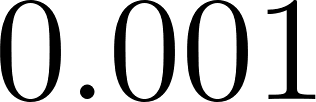 and health is nearly certain at
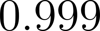 . These are the numbers that a frequentist is unwilling to state and a Bayesian insists on, and they dominate everything that follows.
After one positive test, the posterior for disease is 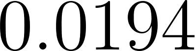 , or 1.94%, and the MAP hypothesis is still
healthy. The test’s 99% sensitivity feels decisive, but the prior is so heavily stacked against disease that a single result barely moves the needle. The healthy posterior is 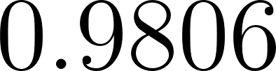 , so the model is not confused, it is appropriately cautious. This is the correct behavior, not a bug in the test.
The coin line reports  and
 for 60 heads in 100 tosses. The observed rate of 0.6 sits exactly two standard errors above 0.5, and the two-tailed p-value of about 0.0455 is just under the conventional 0.05 threshold. That is a borderline result, and the honest reading is “suggestive but not overwhelming.” A larger sample with the same proportion would produce a smaller p-value, because the standard error shrinks with the square root of .
The Wilson interval is the more informative output. It says that the data are consistent with a true bias anywhere from essentially fair to about 69% heads, and it stays inside where the naive Wald interval might not. Reporting the interval alongside the p-value is a habit worth keeping, because the interval carries the uncertainty that a single p-value hides.
Wrap Up
This chapter built three tools in a few dozen lines of dependency-free Scala.
- The Bayesian model, a normalized map plus a two-line update, shows how a prior and a likelihood combine into a posterior and how evidence accumulates across updates. The medical example is the case to remember: a 99% sensitive test yields a 1.94% posterior when the condition is rare, because base rates set the scale.
- The frequentist toolkit builds the normal CDF once and reuses it for z-tests, chi-squared tests, and Wilson intervals. It answers a narrower question than Bayes, requires no prior, and outputs a p-value that says how surprising the data are under a null claim, not how likely the claim is.
- Correlation compresses the co-movement of two series into a single number in
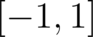 and guards against the degenerate constant case. It measures association, never causation, and only linear association at that.
The recurring theme is that the denominator decides the answer. In Bayes it is the marginal likelihood that lets the base rate dominate. In the z-test it is the standard error that sets the scale of the evidence. In correlation it is the product of the spreads that puts on a fixed scale. When a probability result looks wrong, find the denominator and the intuition usually returns.
The code also shows a style that later chapters reuse. Small immutable value types, companion objects for the operations, pure functions with require guards on the preconditions, and a test file that uses plain assertions instead of a framework. That shape scales from a seven-line Bayes model to a full neural network.
Optional Practice Problems
A better test. Modify
probabilityDemoso the screen test has a sensitivity of 0.99 and a false-positive rate of 0.01 instead of 0.05. Compute the posterior for disease after one positive test and compare it to the 1.94% baseline. Explain in one sentence why lowering the false-positive rate helps so much.Three hypotheses. Extend the medical example to three hypotheses:
disease,healthy, andcarrier, with priors, 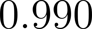 , and
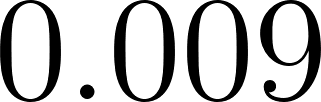 . Give carriers a positive-test likelihood of
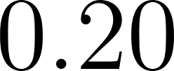 . Run one update and check that the three posteriors sum to one. Which hypothesis is the MAP?
Sequential evidence. Starting from the original two-hypothesis model, update with a positive test three times in a row and print the disease posterior after each step. Confirm the sequence is strictly increasing and report the value after the third test. Is the MAP still
healthy?Odds form of Bayes. Add a function
oddsRatio(likelihood: (String, String) => Double, h1: String, h2: String, evidence: String): Doublethat returnsP(E|h1)/P(E|h2). Use it to show that the posterior odds equal the prior odds times the likelihood ratio, and verify the identity on the medical example.Rejecting the null. Add a function to
Frequentistthat takes a p-value and a threshold and returns"reject"or"keep". Run it on the coin case with 60 heads in 100 and again with 700 heads in 1000. Report both decisions and the p-values.A confidence interval for a proportion of zero. Call
Frequentist.wilsonInterval(0, 20)and print the result. Then compute the naive Wald interval by hand and explain why the Wilson version is the one to trust.
Correlation versus causation. Construct two series with
near 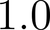 that have an obvious common cause, for example the number of umbrellas sold and the number of puddles in a month. Write a short paragraph explaining why high does not license a causal claim.
Non-linear dependence. Create two series where
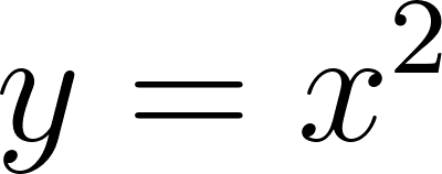 for in
 . Compute
Correlation.pearsonand observe that it is near zero even though is a deterministic function of . Explain what this says about the limits of .